# Examples
- Fast modular exponentiation algorithm
- Euclid's GCD algorithm
# Merge Sort
Best Video showing it in action
# Gauss's idea
This isn't necessarily a D&C concept but can be used while solving fast multiplication D&C problem
Multiplication is expensive
To get the product of two complex numbers:
Since there are four products of real numbers involved (ac, bd, ad, bc), can we lower the number of multiplications?
We can do so by computing (bc+ad) directly without doing the multiplication bit for that part.
Elaboration
Reusing this in the above equation of multiplying two complex numbers, we get
So, due to the modification, now if we compute three real number multiplications: ac, bd, (a+b)(c+d), we can now get product of two complex numbers.
# Fast Multiplication
Multiplying two N-bit numbers where the numbers are large like 1000-2000 bits, we can't use the simple multiplication since the hardware can't handle it. For things like RSA.
Input: n-bit integers X & Y, assume n is a power of 2
Goal: compute
# Naive Approach
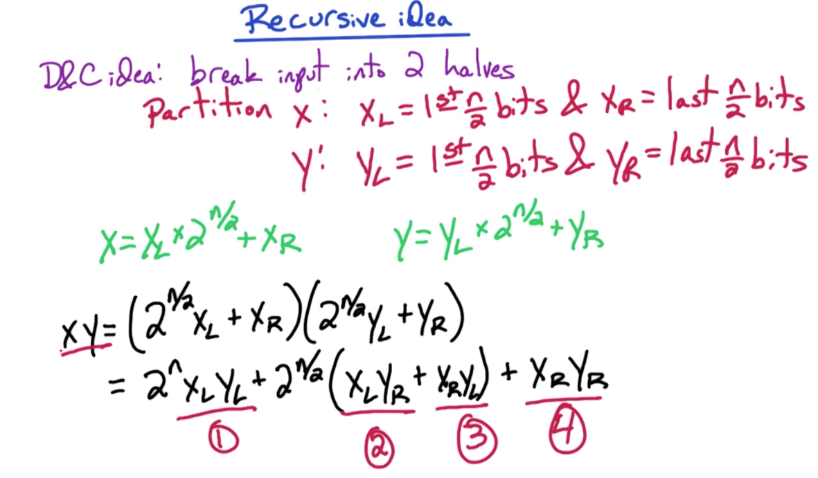
Above, the way X is
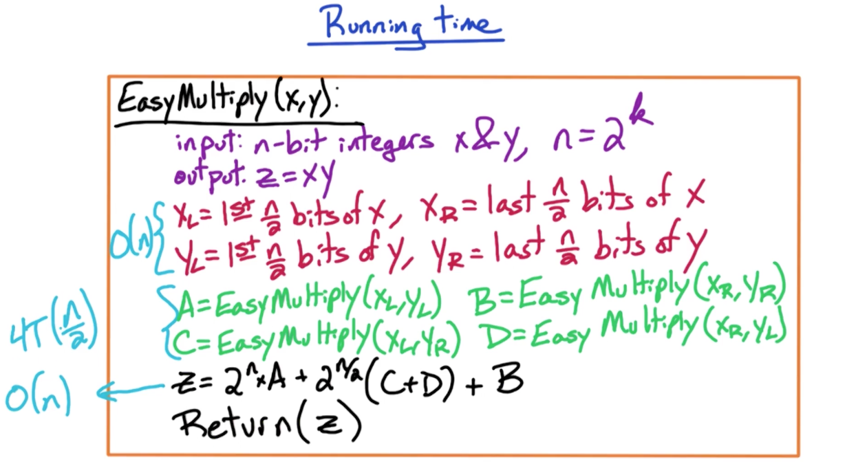
Run time:
Look at Solving Recurrences to understand how this solves to
# Improved Approach
This is where we simplify the above approach using Gauss's idea. We apply Gauss's idea to the part where XY is expressed in terms of
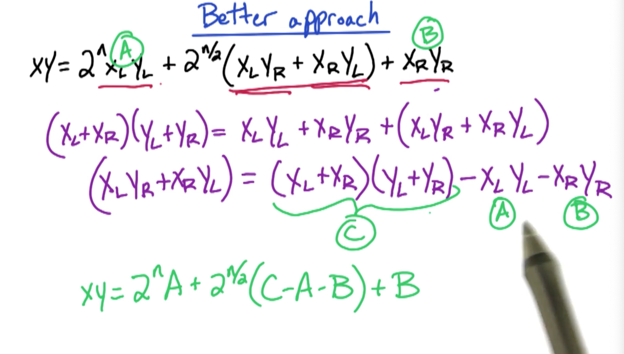
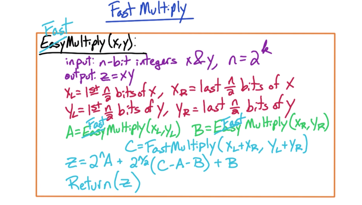
Run time:
The runtime of this improved approach is explained here
# Median
Finding median from a large list of unsorted numbers
A trivial solution with O(nlogn) time complexity is sorting the list and choosing n/2 item for median. But we want something more efficient at O(n)
We are going to leverage a modified version of Quicksort algorithm for this.
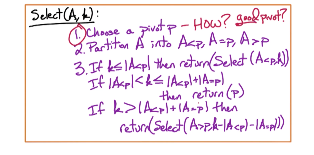
# How quicksort works
- Choose a pivot
p(main challenge) - Partition
Ainto - Recursively sort
The time complexity for quicksort is O(nlogn) but we are going to aim to make it efficient.
# Finding n-th largest element
See below for how we'd pick the n-th largest (k) item using quicksort without fully sorting
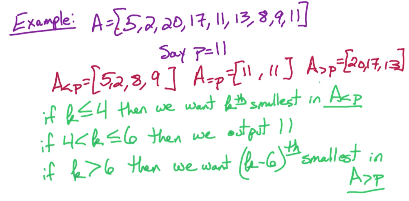
As we can see above, after we partition, we only sort A == p depending on which bucket contains our index of interest. In case of a median, we're interested in k=n/2. So after such a partition, we only zoom in to the bucket that has that index. And we only sort that bucket, and get the value from the index. In the case above, we'd just pick the A==p since it has index 5 and 6 and we'd just pick 11 from there. Of course, the main challenge lies with how to pick the best pivot for partioning.
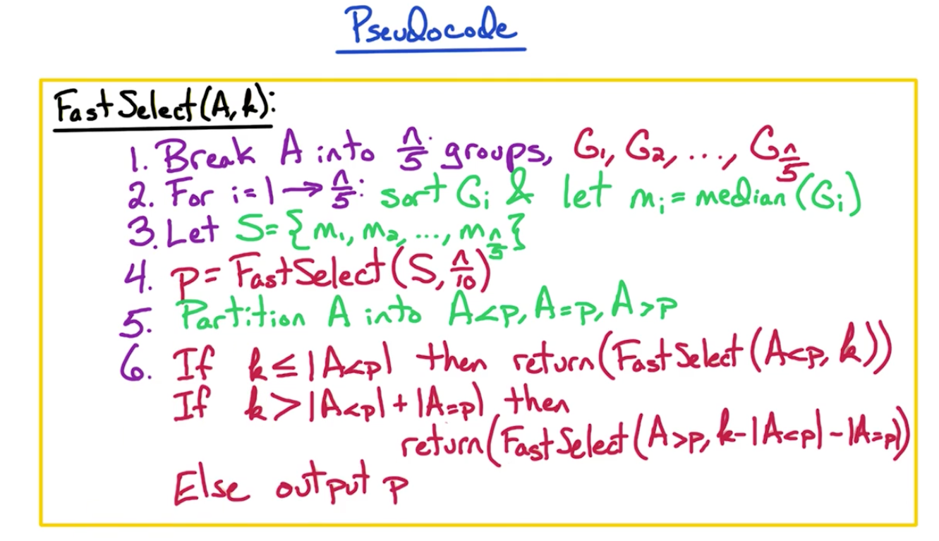
Expressing the above in psedudocode form looks like this:
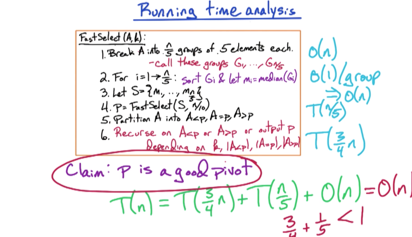
To achieve an 1/b part of the equation dictates how much smaller the input list becomes with every iteration, this means, even if it is not sufficiently small like 1/2 (where b=2), that's fine. We have values like 3/4 (where b = 4/3) and that is fine too, it will still ensure our overall time complexity gets resolved to O(n) using master theorem.
Good Pivot: Therefore, a pivot p is good if
This will ensure a runtime of
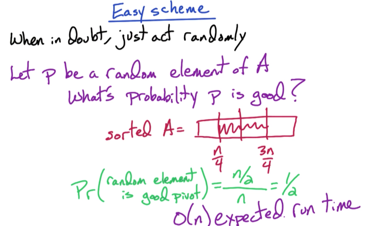
# Good Pivot
We can pick a random pivot and still have a 1/2 probability we will make a good pick, because to fulfill the above runtime, we just have to pick something between
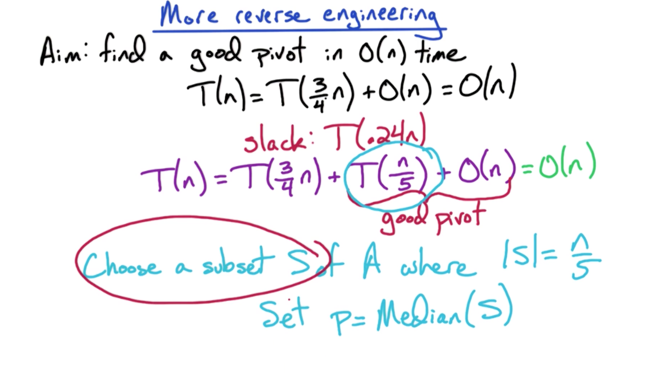
A better approach is outlined below. If we can aim for the sub-problem input size (1/b) to be
Bad approach: The following shows why choosing the first n/5 elements of A as the subset S is not a good idea. Lets assume A is sorted, then choosing S as the first n/5 elements of A means:
- S =
n/5smallest elements of A - P =
n/10th of smallest element.
So the subproblem doesn't decompose by much as most of the partitioned elements fall in the `
Good Approach: We need to choose S such that it is a representative of A. We want median(S) to approximate median(A).
- Break A into n/5 groups of 5 elements each. (choosing 5 because we have to do this using the extra bandwith
discussed above to still be at O(n) runtime collectively. We can only break up problems so subproblem input is 1/5 of original input) - For each group:
- Sort the elements within each group and take the median of each group (performance boost here in sorting since this is O(1) due to each group having too small number of elements)
- Continue this recursively and eventually we get a median.
# Pseudocode
# Fast Fourier Transform (FFT)
# Useful resources
Concise Explanation by Sai Sandeep
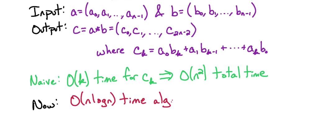
# Problem Definition
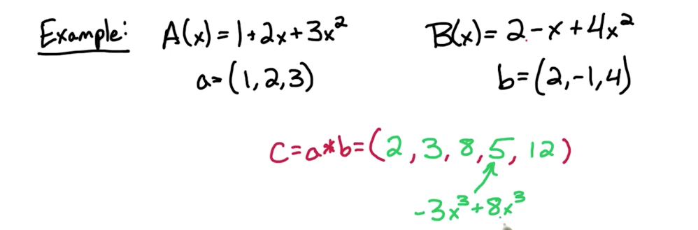
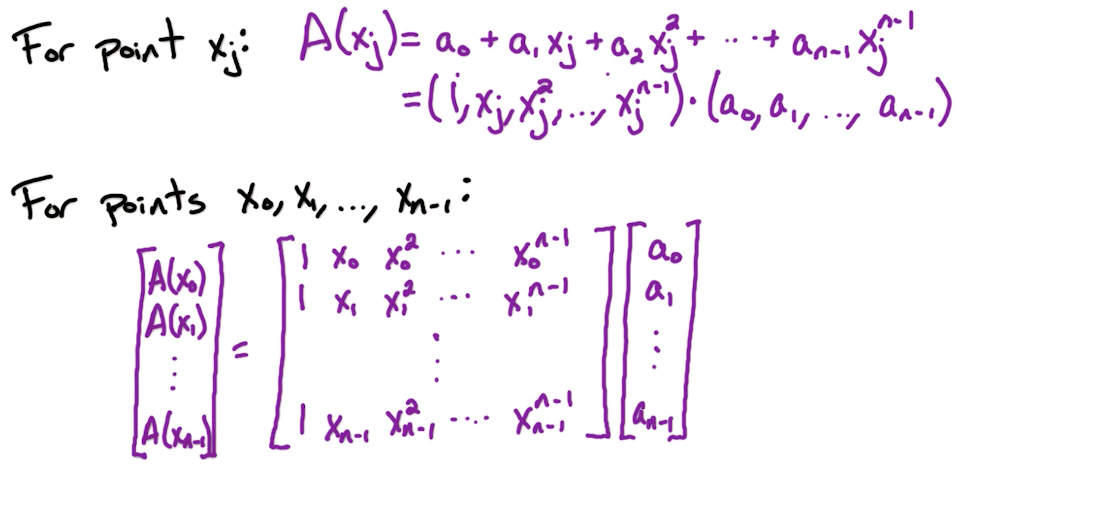
# Polynomial basics
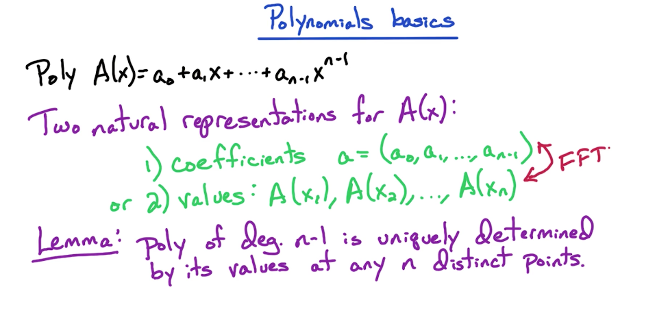
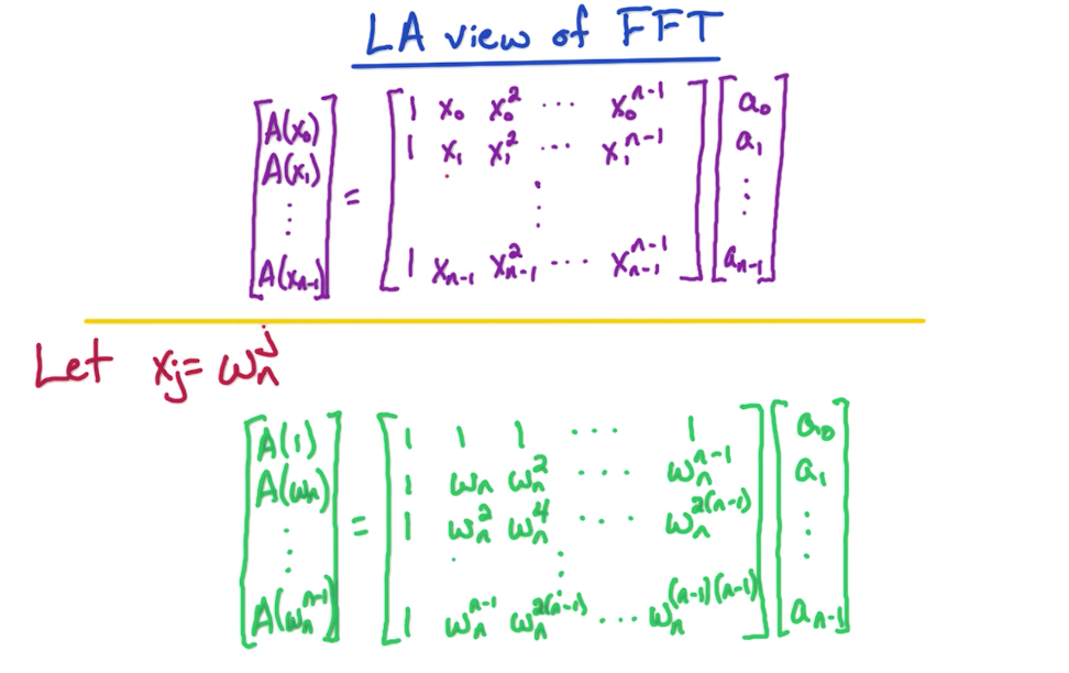
FFT allows us to convert from coefficient-form to values-form and vice versa. The benefit of values-form is polynomial multiplication is more efficient in this form, but the benefit of coefficient-form is a convenient/better way to represent a polynomial. Important point to note is that FFT converts a polynomial from coefficients to values but not for any choice of x1...xn but for a particular well chosen set of points, x1...xn. Now what points do we choose? That's the beauty of FFT explained below in FFT: Opposites section and Complex Roots
We can compute
To validate how Lemma works, lets think of a Line. A line is a degree 1 polynomial (mx + c has only 1 power to x), so it can be represented by 2 points. A triangle is a degree two polynomial and can be represented by 3 points.
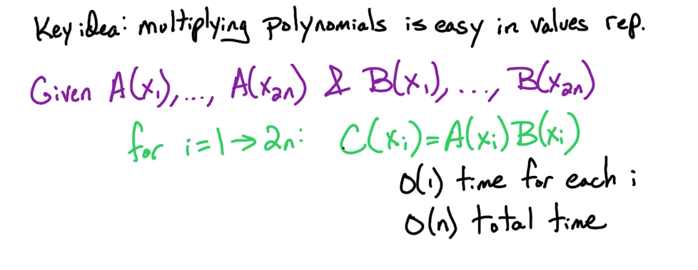
A and B have to be padded before multiplication so it has enough degrees as there would be in C after multiplication.
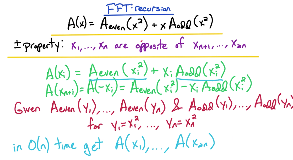
# FFT Opposites
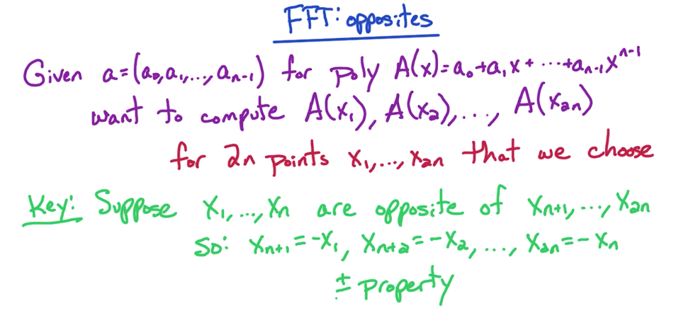
+- property:
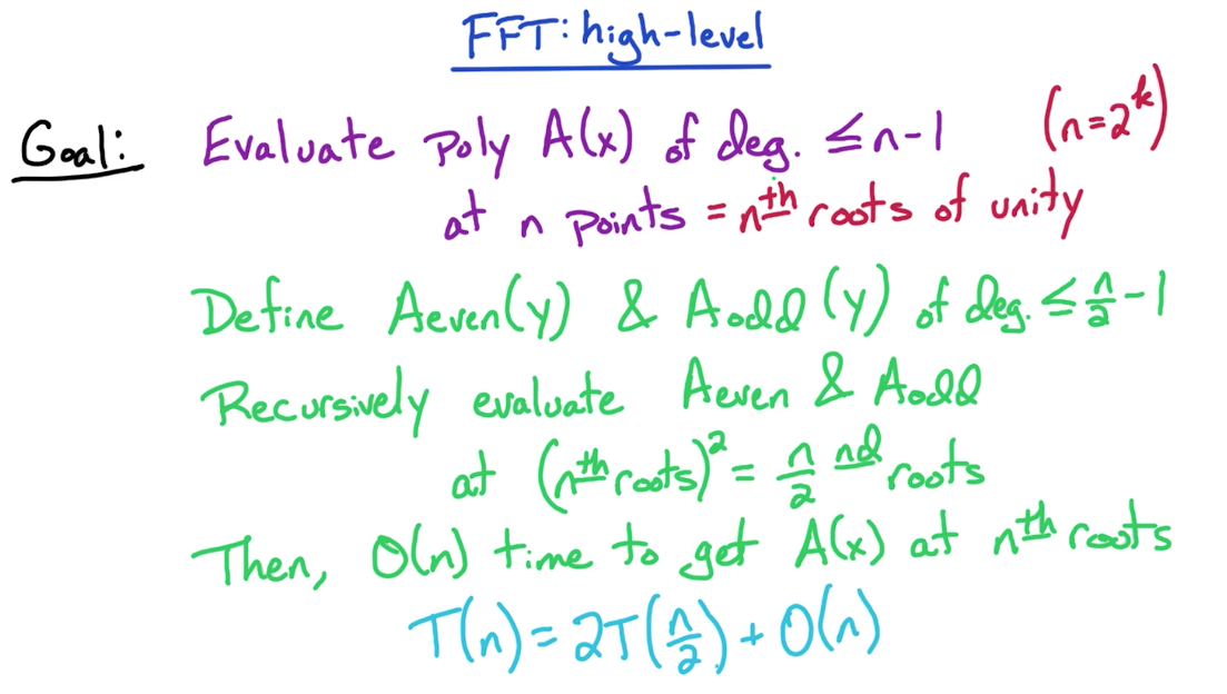
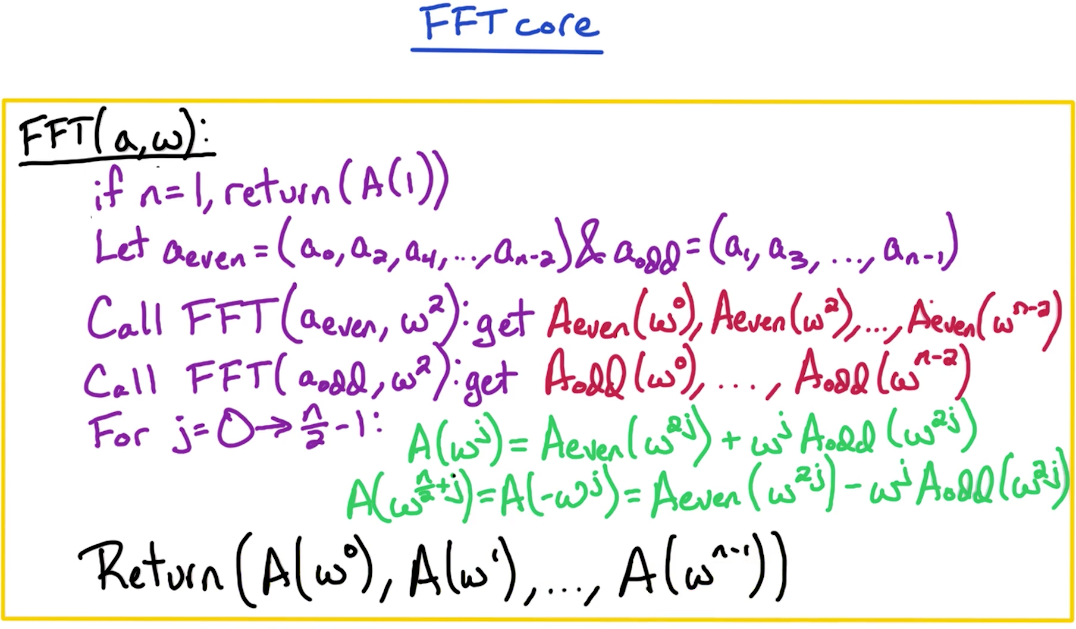
# FFT Even & Odd
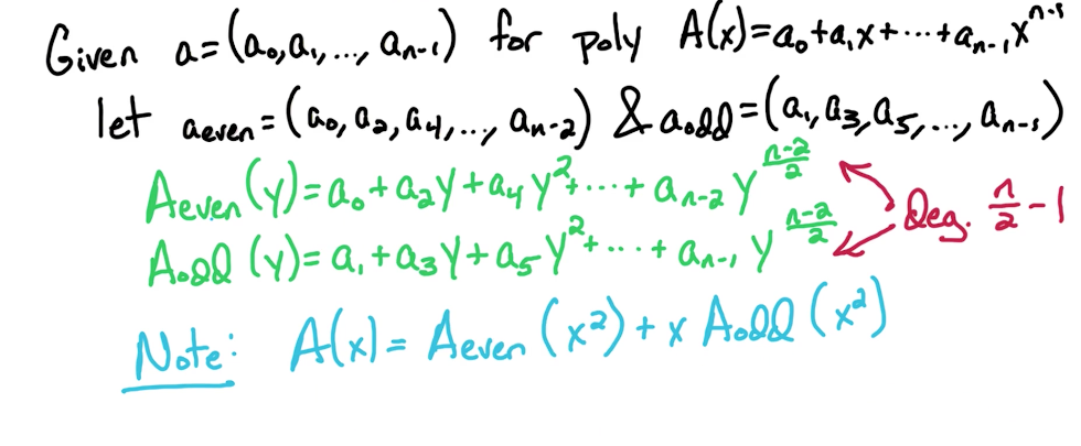
We split the odd and even items from the polynomial. When split, we use the powers of y in the splits to express continuous power. So basically,
# FFT Recursion
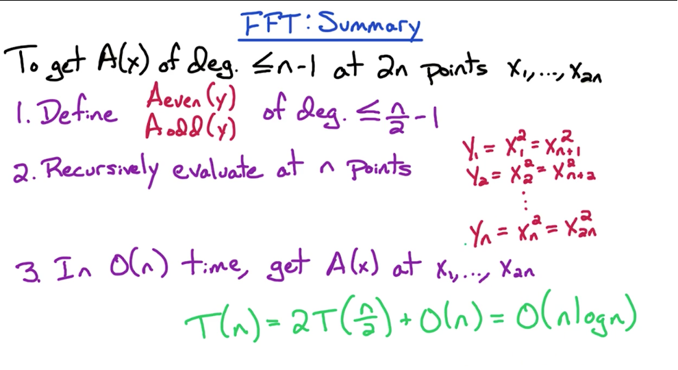
# FFT Summary
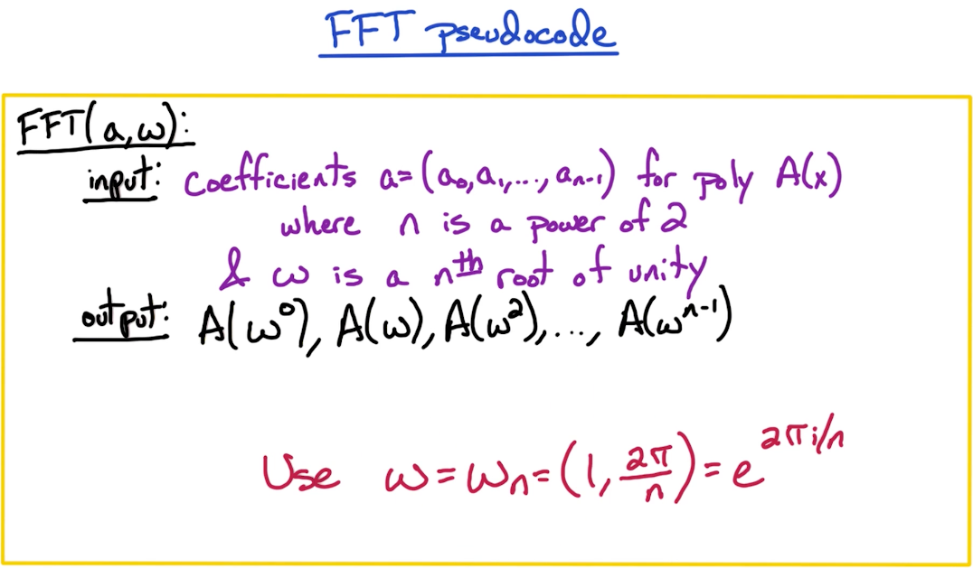
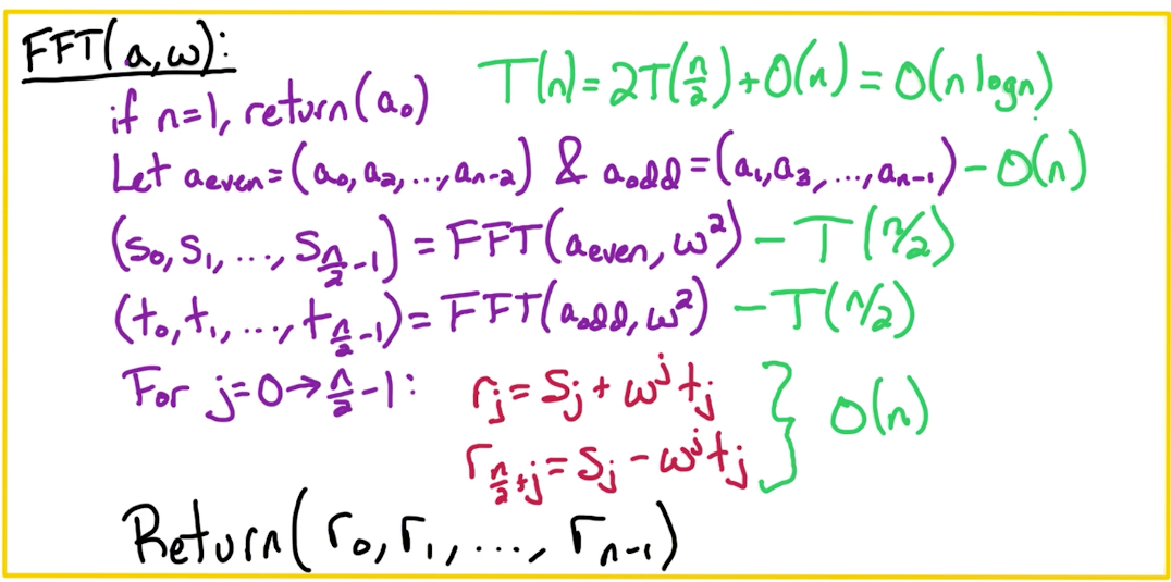
# FFT Algorithm Pseudocode
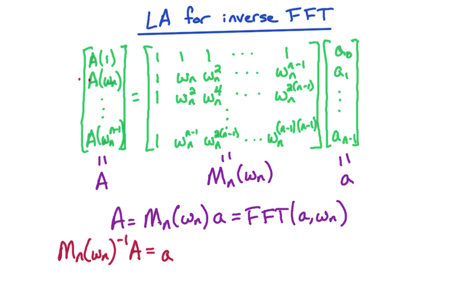
# Linear Algebraic View
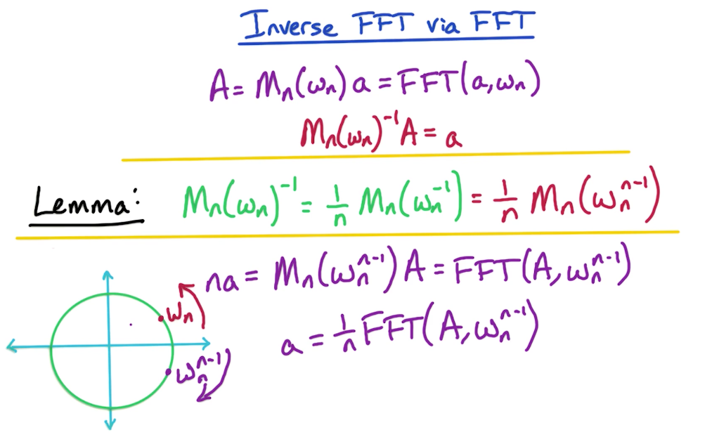
# Inverse FFT
In the first line below, we see the way we compute FFT.
Then after that we are modifying that same equation to yield inverse FFT but using the same function
# Complex Numbers
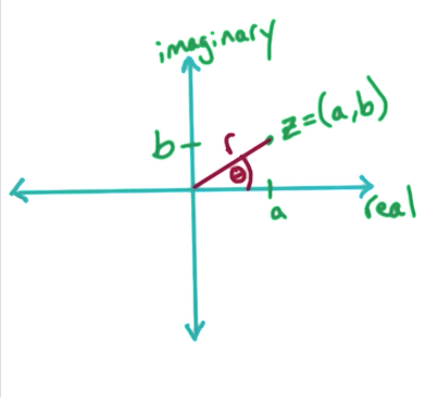
# Polar coordinates
A complex number
Euler's Formula:
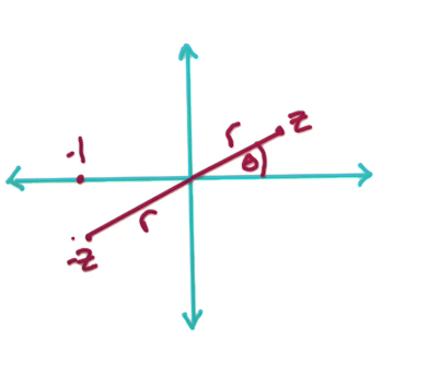
Polar coordinates are a better representation for our purposes for multiplication.
Polar is convenient for multiplication
If we want to compute,
# Complex roots
n-th complex roots of unity are defined as those numbers z where
Examples
Deriving formula for n-th root
since
so this means,
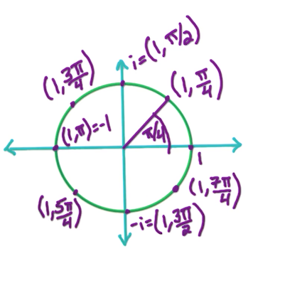
Therefore, n-th roots of unity can be computed so that r is always going to have a constant value of 1, and the theta is going to change based on the value of n which would be problem-specific, and j which is going to be sequential
Below is an example of computing 8-th roots of unity.
Notice that there are n-distinct values, and after hitting n, the values would start to repeat since the roots are in a circle.
The n-th roots are represented using
and likewise
Formula 1: Making the general form to be
Tip: If a question asks to compute
Basically, we divide the circle into n pies (think pie chart) and that is the visual representation of the n-th roots of unity. If you need to get lets say n + 1 or 2n roots, then you just loop over this circle again and again. In the visual example shown above where we got 8th roots of unity,
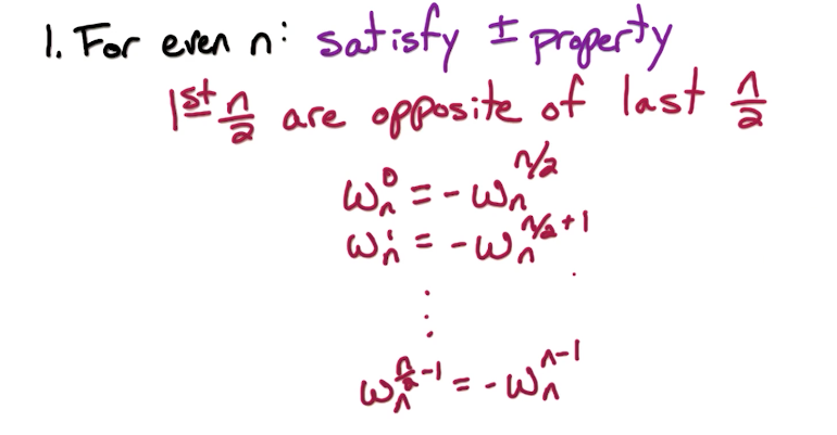
Formula 2: Another useful formula of +- property is:
Formula 3: Using Euler's formula from above,
Below we can see how the different roots compare to each other for the various values of n, and also reflections of one another.
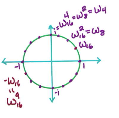
Tip: If lets say
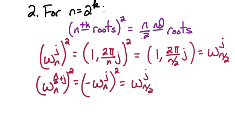
# Key properties
The key properties of n-th roots of unity that we utilize are below.
# Complex Roots Practice
# Solving Recurrences
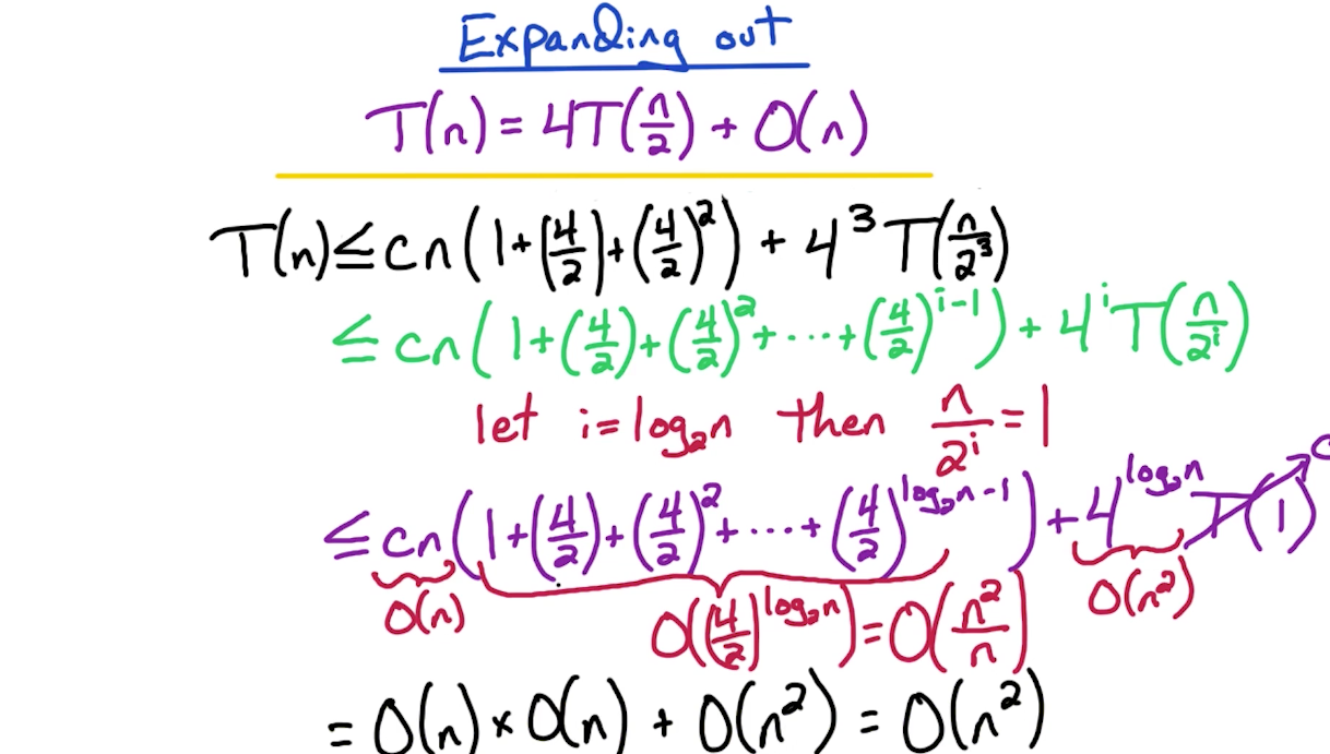
# Expanding out
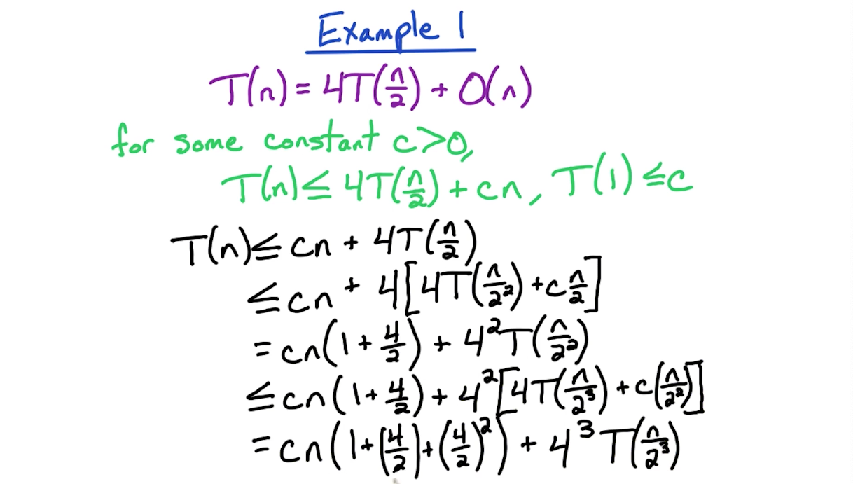
Note: While expanding out, don't simplify the power of something and leave them as is. This helps create the geometric series later to solve.
Notes:
- When do we stop expanding? We stop when the expression inside
T(?)becomes base condition i.e. 1. In this case, when. This happens if .
Proof
The
has suddenly arrived by using the formula/mapping/technique described below in Geometric Seriessection. You might notice the power should bebut that -1 is ignored since it is insignificant while converting to big O terms. Once that is done, it is eventually convered to O(n)using this breakdown:The second half
is solved by the technique described below in the Mapping polynomialsection. On a separate note, the previous bullet point also attempts to solve a similar thing, for which we can use the same understanding of how logs operate.
# Geometric Series
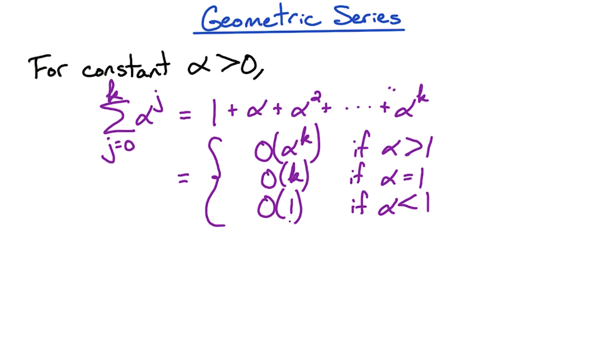
- The alpha > 1 scenario is seen in the recurrence analyzed above for the Naive Fast Multiplication.
- The alpha = 1 scenario is seen in merge sort
- The alpha < 1 scenario is seen in median finding
# Manipulating Polynomials
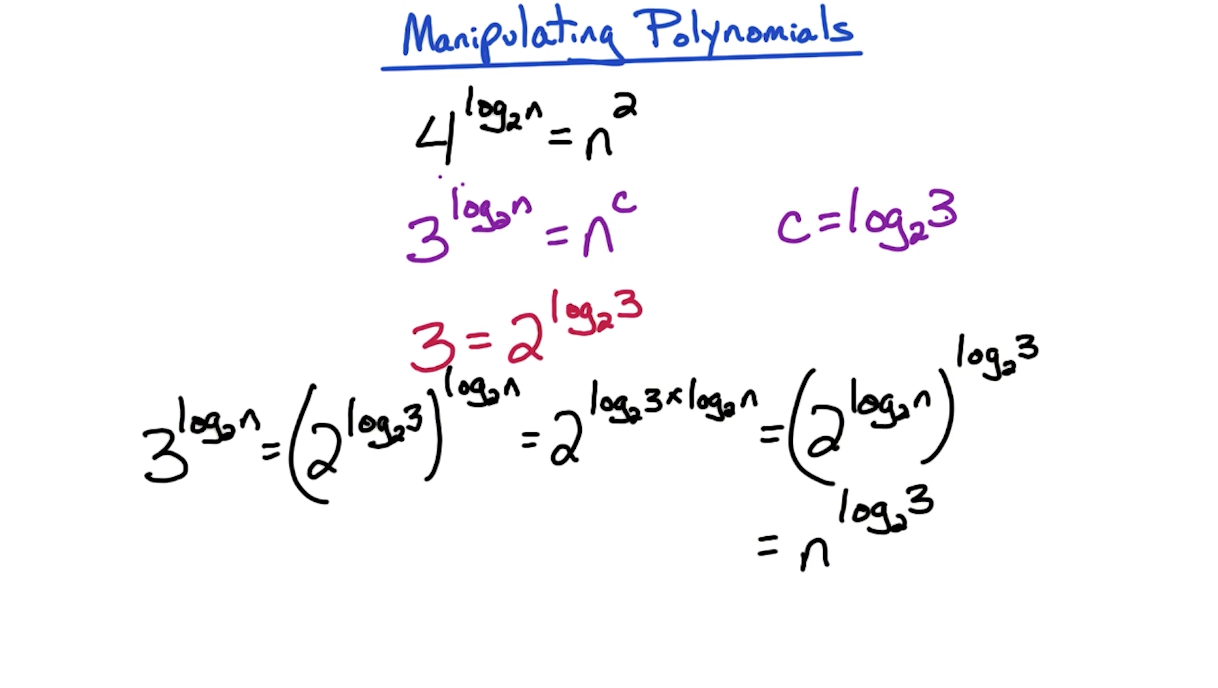
We want to express polynomials in form
To do so, since the base of log is 2, we want to convert the overall polynomial from the
To do this, 3 can be written as
So quick calculation can also be done like this
# General Recurrence
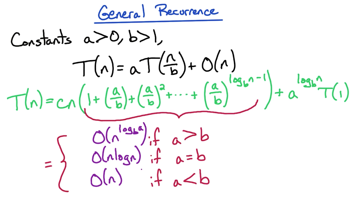
# Examples
# E.g. Merge sort
We partition the list to two: each of n/2, and sorting each is T(n/2). Since there are two partitions, it becomes 2T(n/2). Then merging it back takes O(n).
# E.g. Fast Multiplication: Naive
- Had 4 subproblems, therefore 4T
- n items were divided to n/2 each time, and hence the n/2.
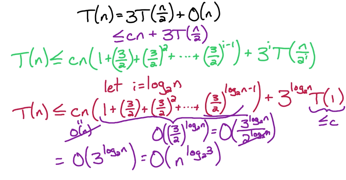
# E.g. Fast Multiplication: Improved
- Had 3 subproblems, therefore 3T
- n items were divided to n/2 each time, and hence the n/2.
# E.g. Median
Runtime:
← Shortest Paths Math →