Linear programming is a general technique for solving optimization problems.
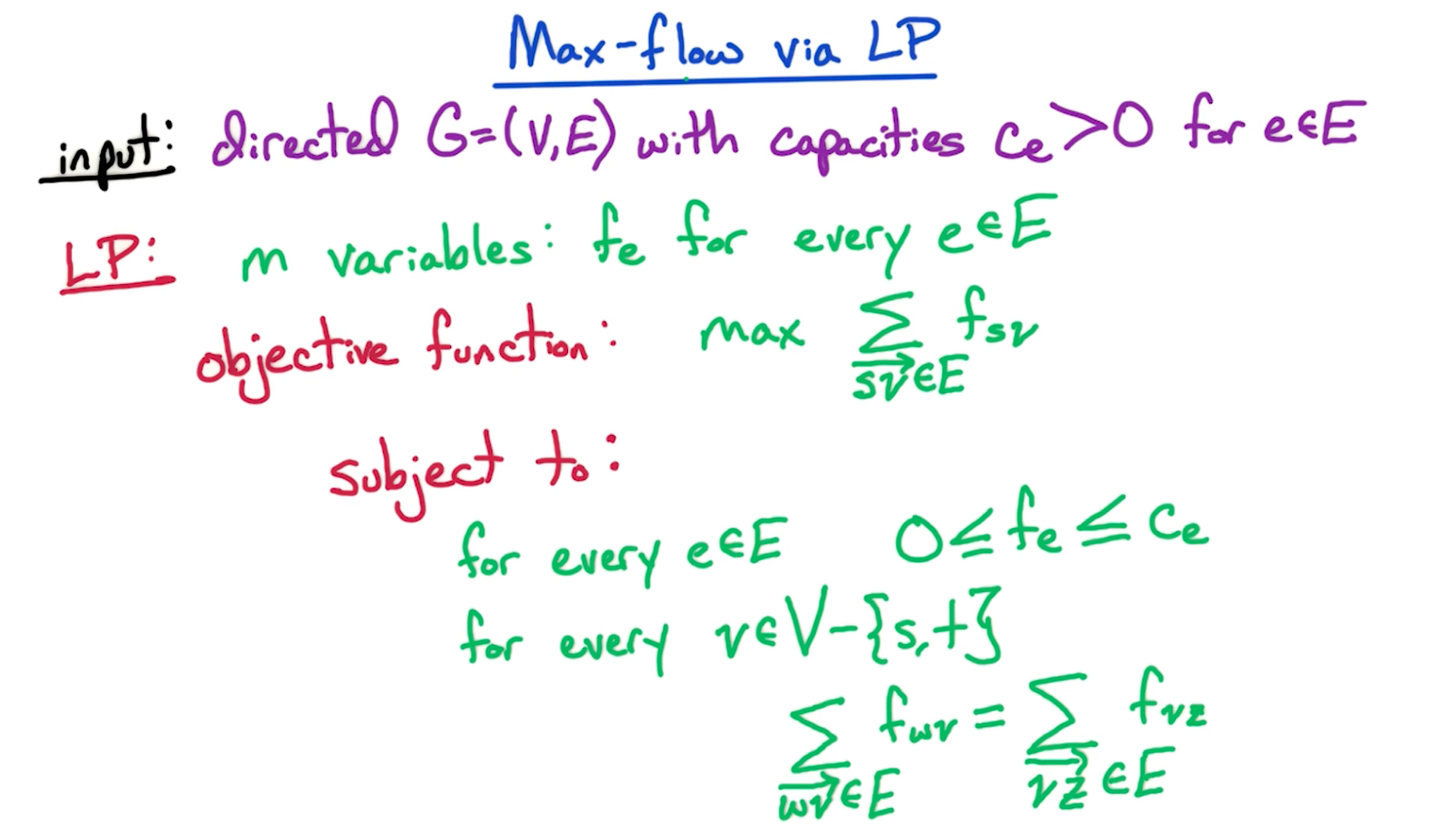
# Max-Flow as LP
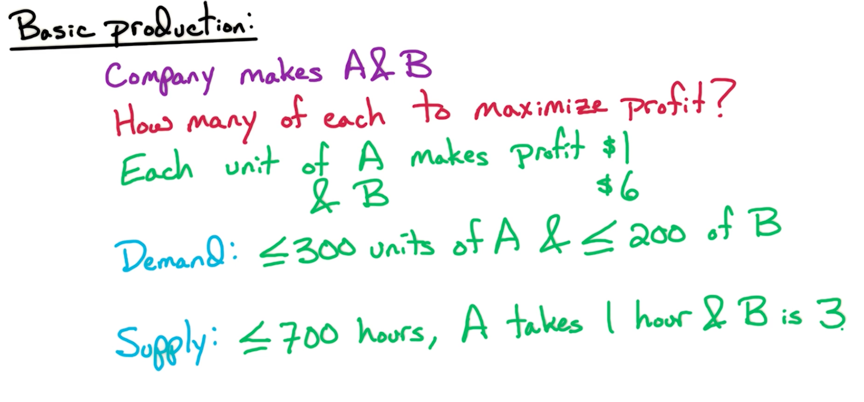
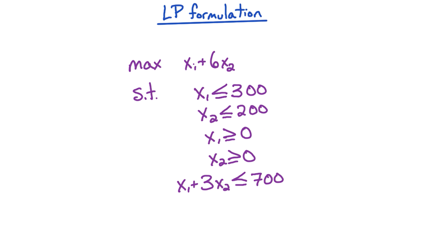
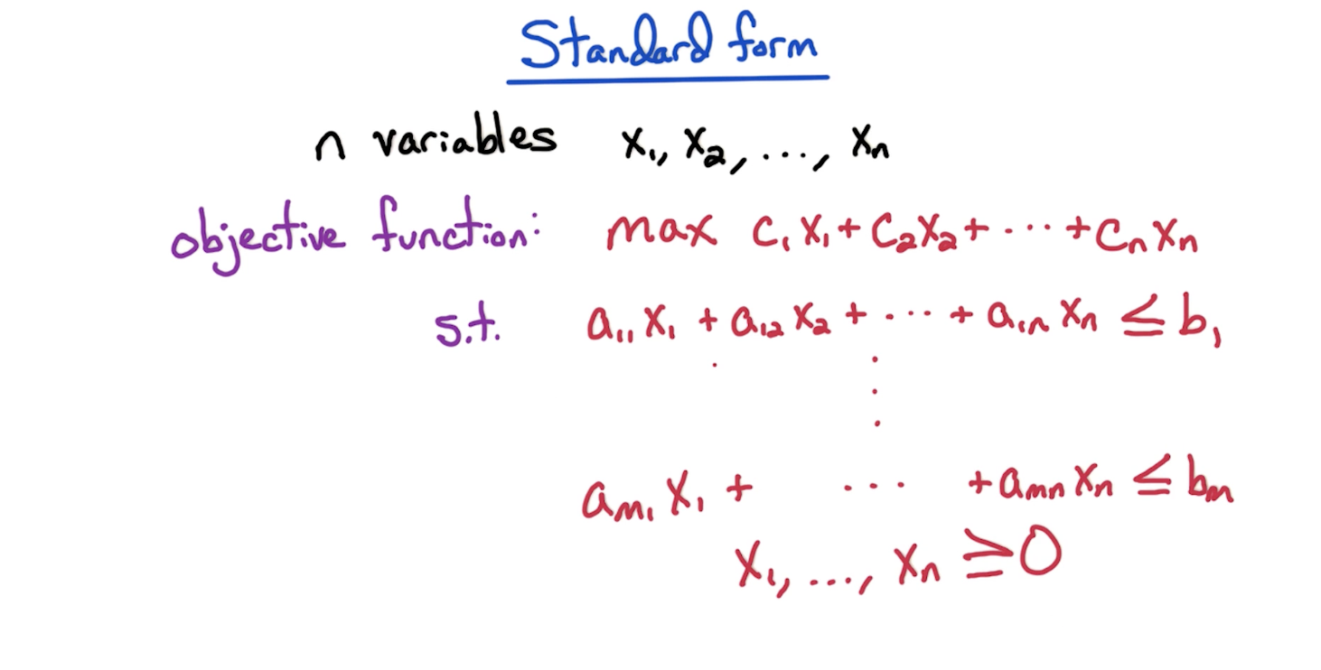
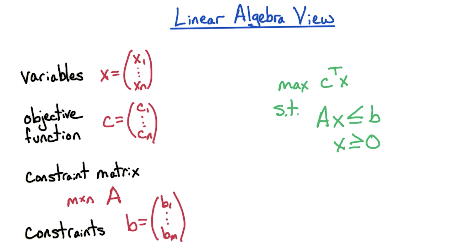
# Basic LP Formulation
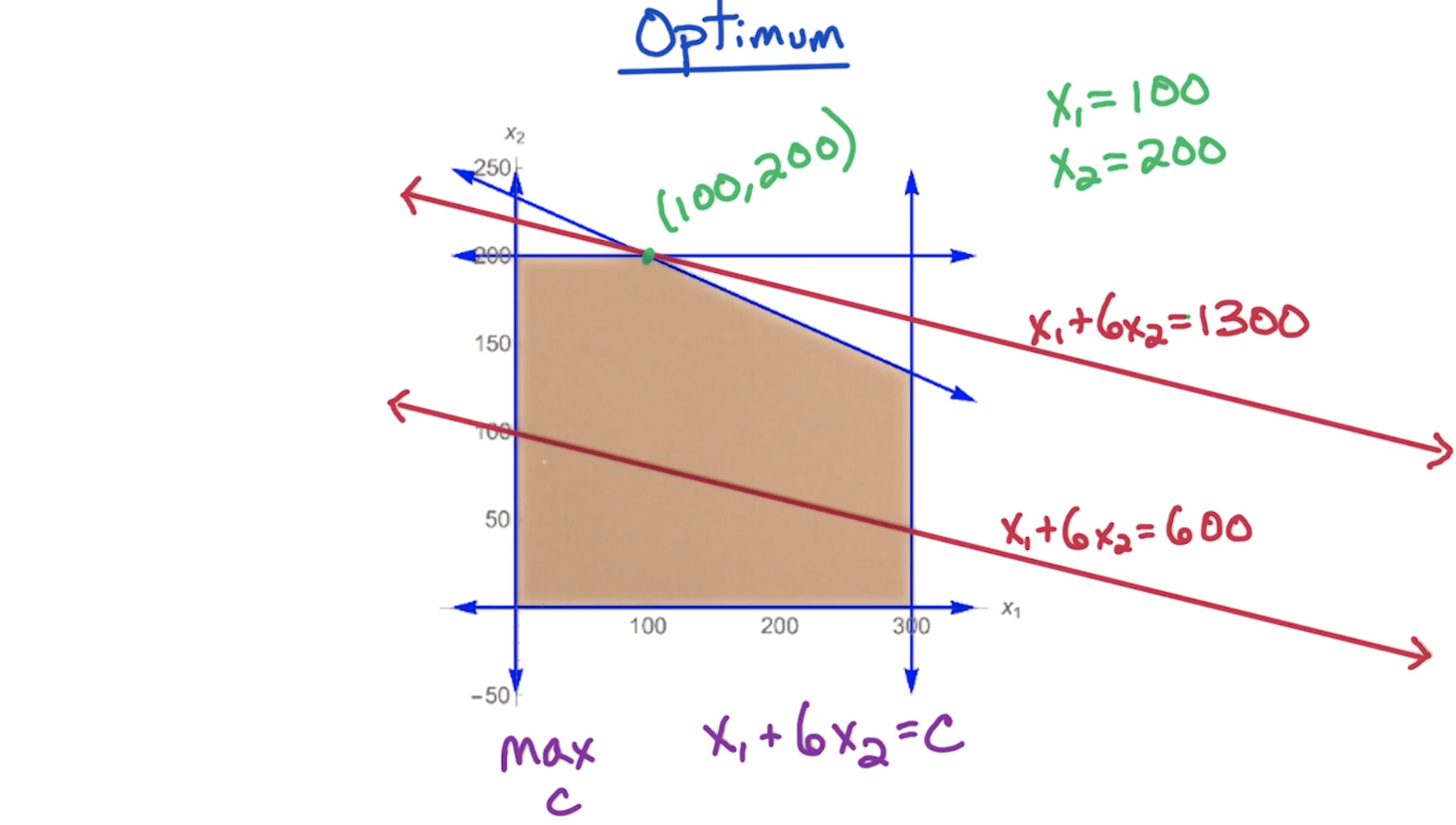
The enclosed/convex region of all these
# Key Points
- The optimal point lies on one of the edges that encloses the feasible region except if LP is infeasible or unbounded
- Optimum may be non-integer, so we could try to round it.
- Linear programming optimizes over the entire feasible region, which can be done in polynomial time, therefore
- Integer Linear Programming is NP-Complete, so it is unlikely we can solve it in polynomial time.
- Optimal point always lies in the vertex of the feasible region
- If a vertex is better than its neighbors, then it is the global optimum.
- Feasible region is convex, which means, if we draw a line between two random points within the feasible region, the line doesn't go outside the feasible region.
# Standard Form
# Converting
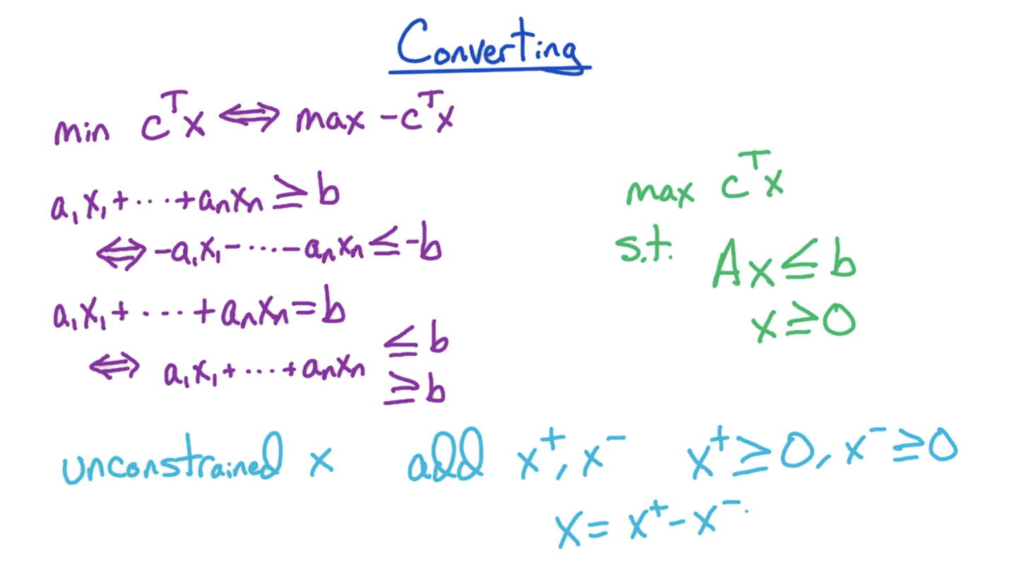
- If you need to convert a maximization problem to minimization problem or vice versa, change the signs of the objective function coefficients.
- If you need to change a greater-than to a lesser-than equation or vice versa, change all the signs on both sides of the equation. Changing to lesser than is required for an equation to be a constraint of a maximization problem.
- If you need to convert an equals-to equation (and this is necessary for it to be constraint of max/min problem), then just create two copies of the equation by replacing the equals-to with a greater-than and a lesser-than sign. Then, for it to fit the max problem requirements, you need to convert the greater-than equation to a lesser-than by using rule from above i.e. changing signs on both sides of the equation.
- Strict inequalities are not allowed in linear programming
- For unconstrained x, ....
# Calculating Vertices
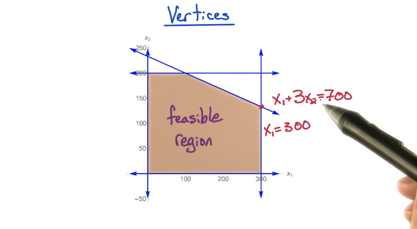
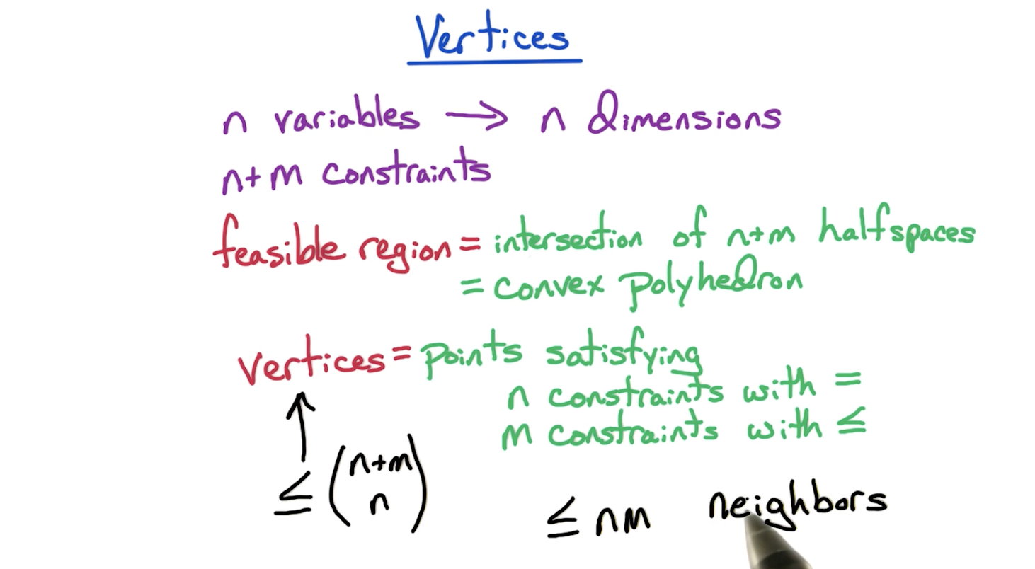
- In the (n+m) constraints, the n constraints refer to the x > 0 kind of constraints for each vertex.
- In the above basic example, since n = 2, we tried using two constraints with equals-to sign to compute a point, and verify that the point satisfies other constraints.
# LP Algorithms
Two polynomial-time algorithms exist
- Ellipsoid algorithms (mostly for theoretical interest)
- Interior point methods (Simplex is an example of this)
# Simplex Algorithm
Worst-case exponential time but it is widely used because the output of simplex algo is guaranteed to compute optimal time and it is very fast for HUGEE LPs.
- Start at some feasible point i.e. x = 0 since this falls within the feasible region due to there being
nnon-negativity constraints and hence is a vertex. - We need to check the point satisfies other
mconstraints. If it doesn't satisfy any of themconstraints, we know this point is not in the feasible region and therefore the feasible region is empty. This LP is infeasible and we're done. - If it satisfies the
mconstraints, lets move further. Look for neighboring vertex with higher objective value.- If we find one, we move there and repeat from step 1 by using that point as the new feasible point. If multiple better points exist, we can go by picking one randomly, or pick the highest objective value point.
- If no better neighbors exist, the current point is guaranteed to be the best point and hence we return this as output.
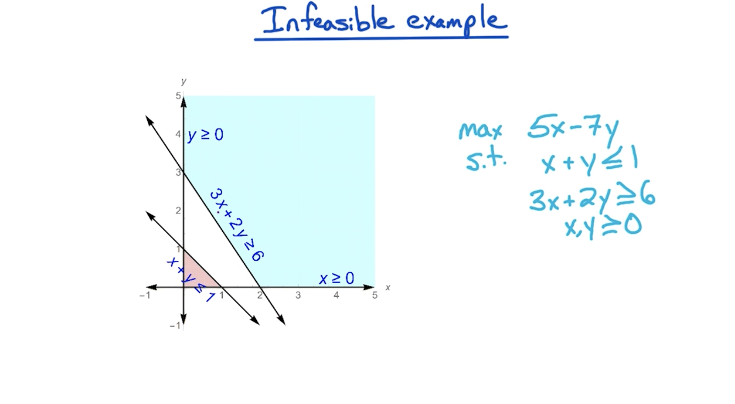
# Infeasible
LP being infeasible means the feasible region is empty
Tip: The objective function has nothing to do with making an LP infeasible, it is the constraints that are responsible.
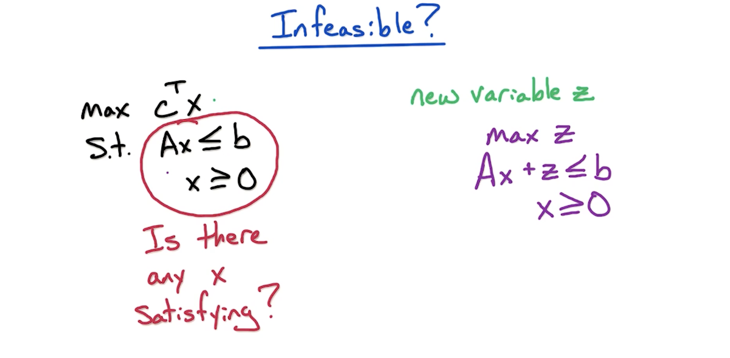
To find out if an LP is infeasible, we create a new LP with constraints that has an added variable z variable added to the constraints. We maximize for z. If the optimal value of z is non-negative, we know original LP is feasible, otherwise, infeasible.
# Unbounded
LP being unbounded means optimal is arbitrarily large.
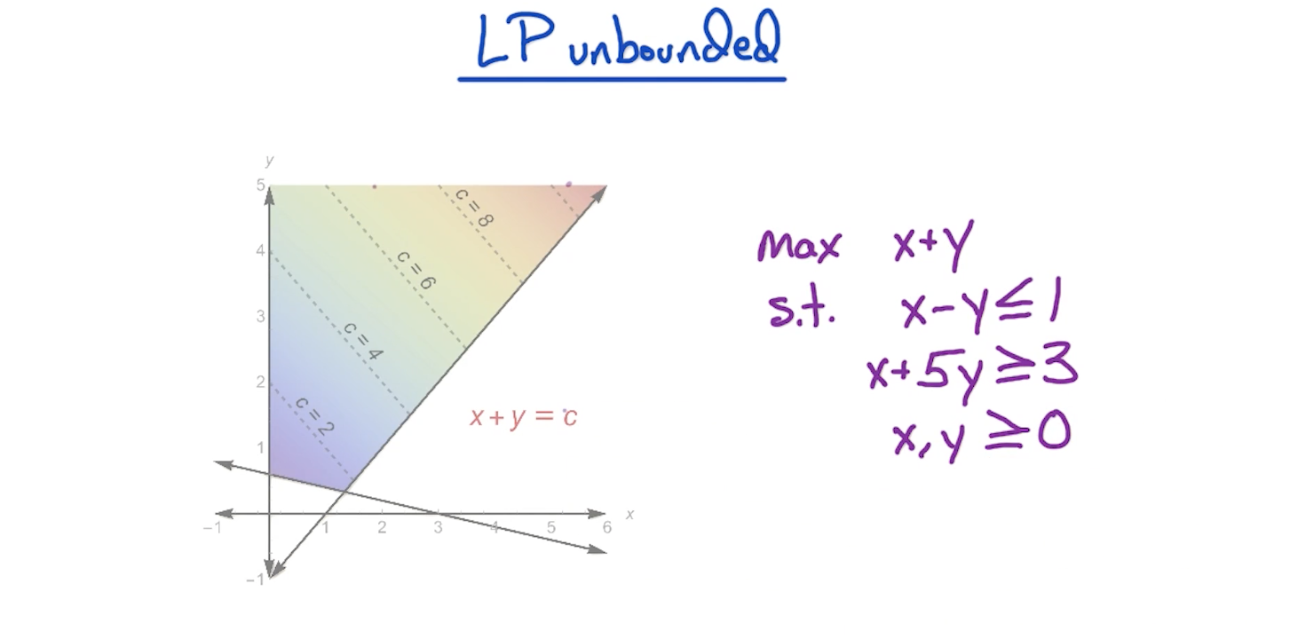
There might exist an objective function for which the optimal is achieved at lower regions given the same constraints.
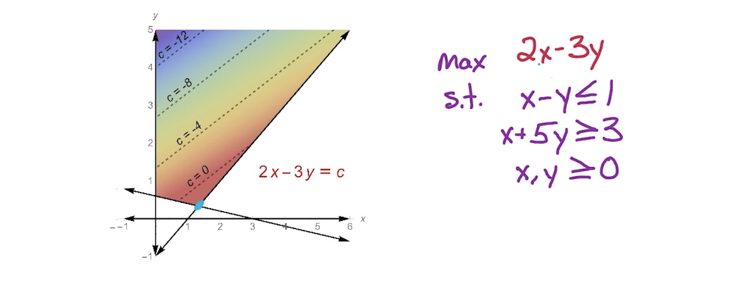
In this case, even though the constraints are the same, we are able to achieve the optimal value due to the objective function.
Tip: To figure out if a feasible LP is unbounded or bounded, we have to look at Dual LP. Look at Weak Duality below
# LP Duality
Assuming someone gives us a value saying it is the optimal solution to an LP problem, we can verify using LP Duality.
We can do so by getting the upper bound of the LP. How do we do this?
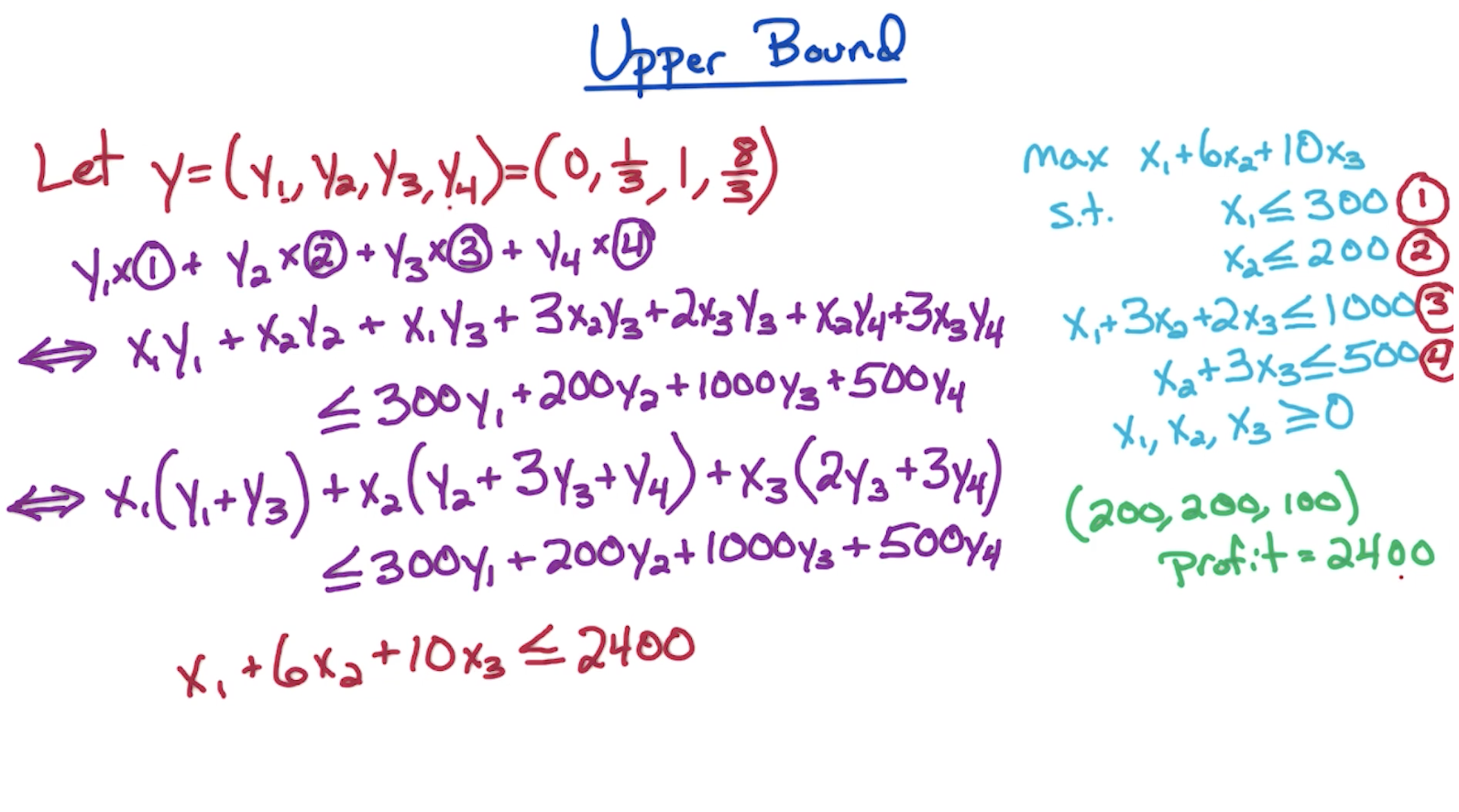
# Upper Bound
Explanation
- We need the Y vector with the number of dimensions equal to the number of constraints of the LP i.e. 4 in the following example. We'll figure out how we got the values for the 4 dimensions
later. - Then we multiply the Y vector with the respective constraints. i.e.
on both sides of the inequalities - Then we plug in the values of the all the
and we should get an output that looks like - The LHS doesn't have to be exactly the objective function but at least as big as the objective function i.e. in the above case, it could've been
Therefore, we verify that the UpperBound is the optimal solution for the LP
# Computing Y vector
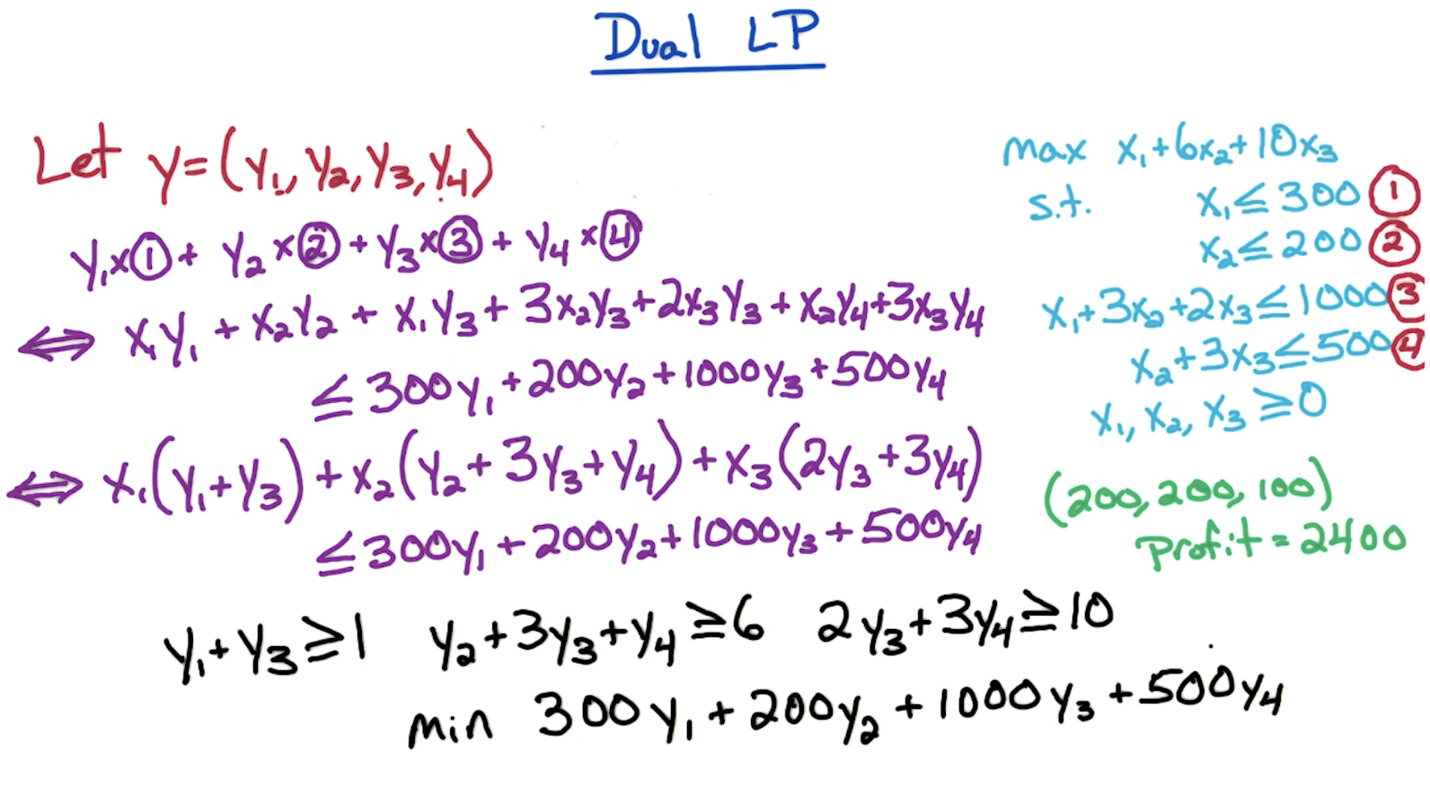
We can reverse-engineer the value of Y vector from the last step of computing the upper bound above.
Since in the last step of the above process, we need LHS to be as big as the objective function, we need coefficients of
The RHS will serve as the upper bound on the LHS and will also be the upper bound on the objective function. And we want to get the smallest possible upper bound, hence minimize.
Therefore, computing Y becomes a minimization LP problem of itself, where the RHS is the objective function which needs to be minimized, and the constraints are ensuring coefficients of
In short,
- Coefficients of LHS define the LHS of constraints
- Coefficients of the original objective function define the RHS of constraints
- RHS of original constraints define the minimization objective function of Y vector.
I guess this is why it is called the dual LP, since we are performing another LP to verify the solution to the original LP is correct.
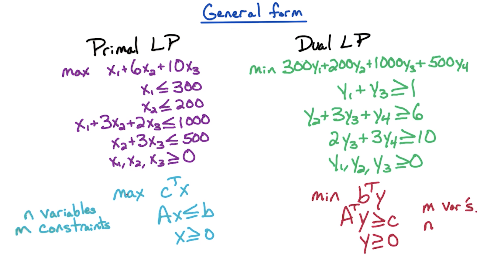
# Cheatsheet to construct Dual LP
- Number of variables in the original LP = number of constraints in the dual LP.
- Number of constraints in the original LP = number of variables in the dual LP.
- If RHS of original constraints are 300, 200, 1000, 500, dual LP objective function is
- If coefficients of original LP objective function are (1, 6, 10), dual LP constraints have RHS of 1, 6 and 10 respectively.
- If
is present in the first constraint of original LP with coefficient 10 and third constraint of original LP with coefficient 20, then the second constraint of dual LP is .
Refer to the following for these cheatsheet ideas going into effect.
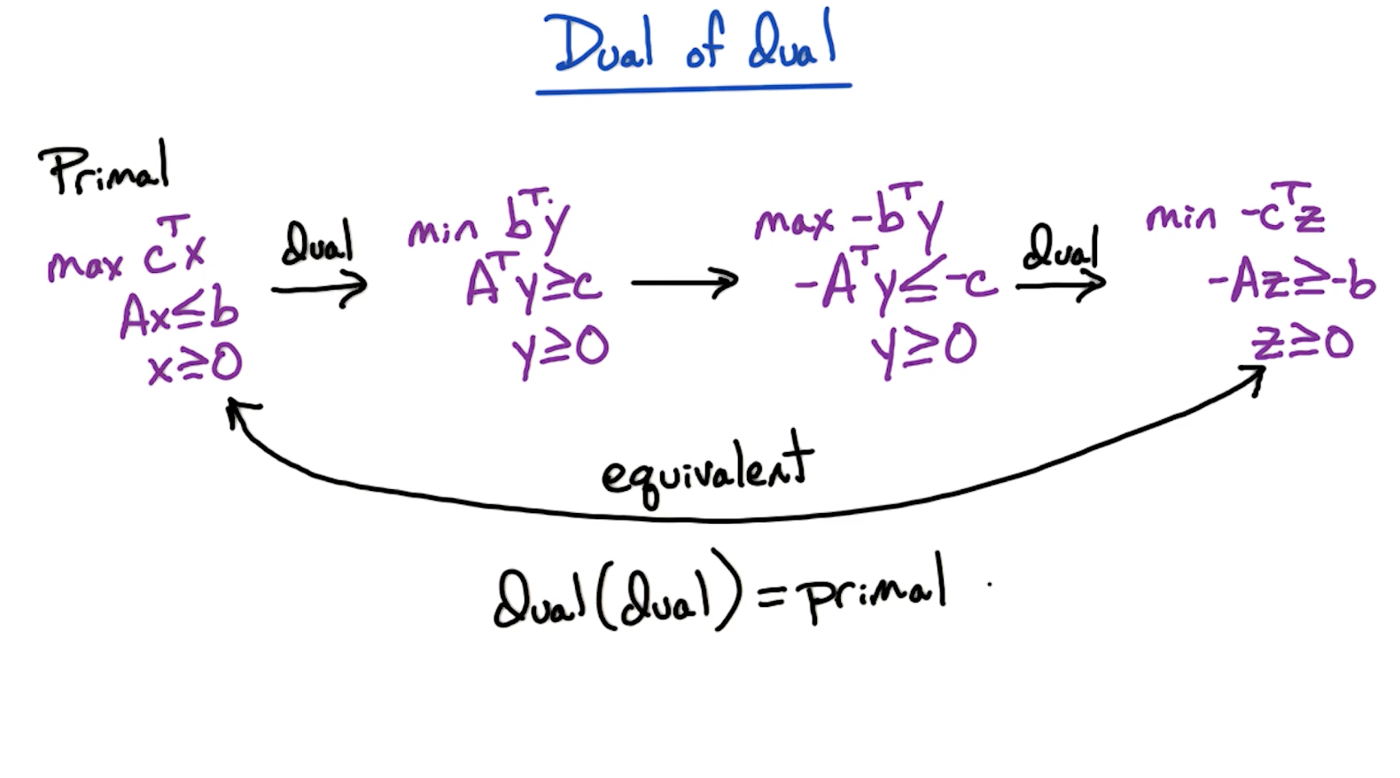
# Dual of Dual
Important: You should convert any LP to standard form (maximization problem with <= constraints) before attempting to compute the dual of it.
# Weak Duality
The Dual LP gives the upper bound of the primal LP.
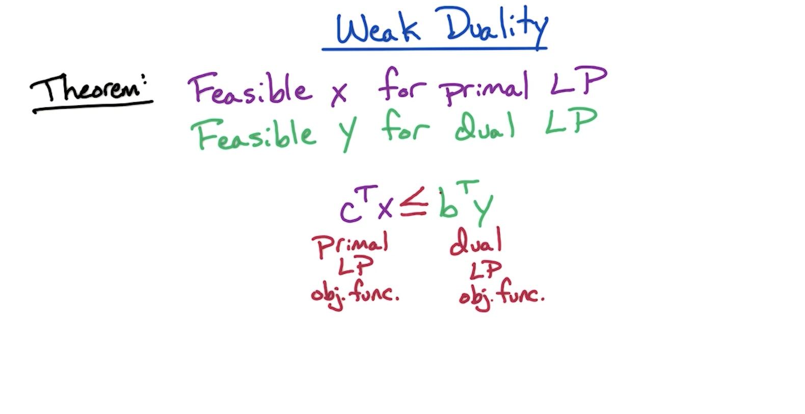
Corollary 1: If we can find feasible x and feasible y where x and y are optimal.
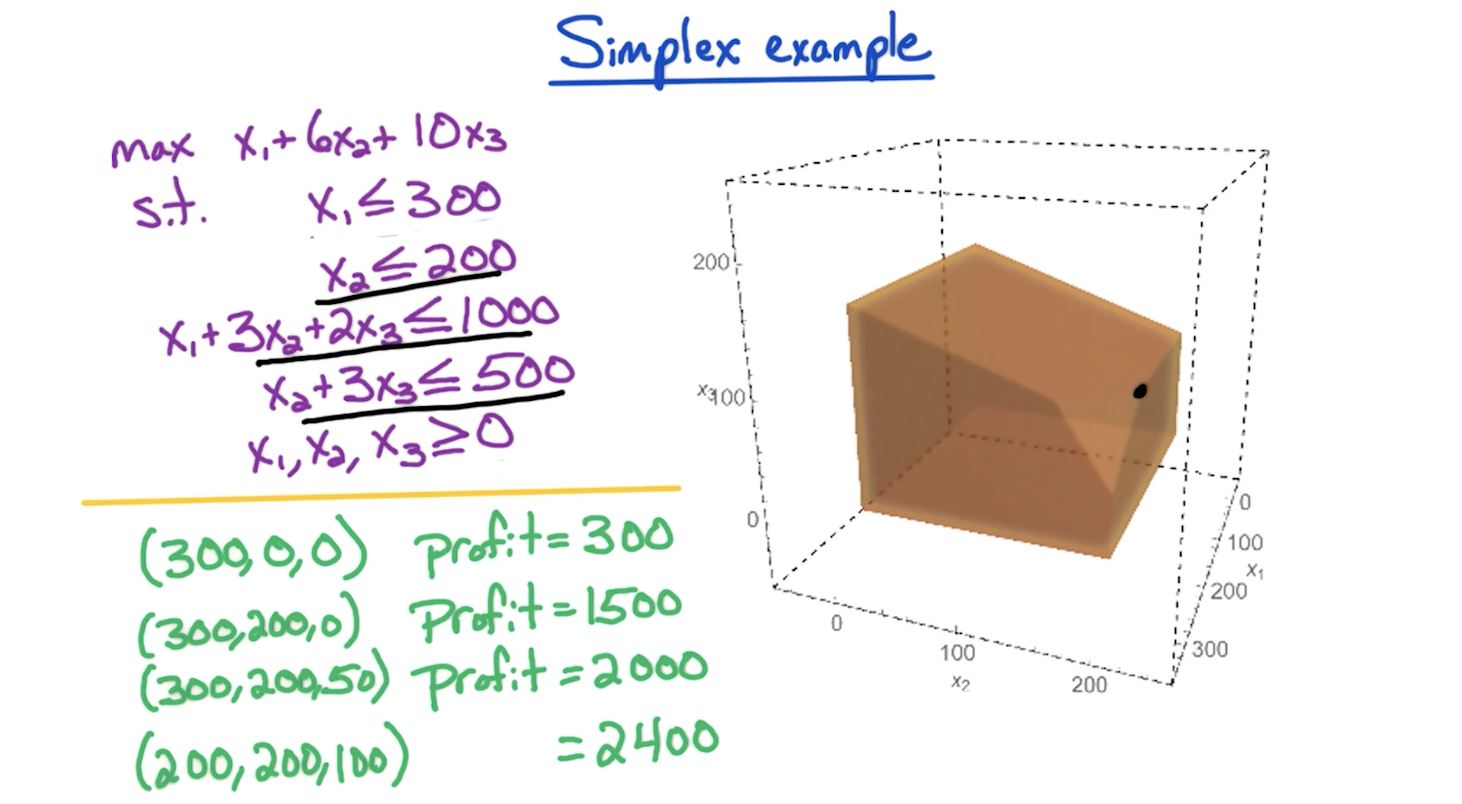
We achieved this corollary in the earlier example where we got solution of primal LP as 2400.
Corollary 2: If primal LP is unbounded, then dual LP is infeasible. If dual LP is unbounded, then primal LP is infeasible.
Notice that this is not iff. It is possible both primal and dual is infeasible. Also possible, if dual is infeasible, primal might be unbounded or infeasible.
Therefore, to check if a primal LP is unbounded
- First we check if primal LP is feasible.
- Then we check if dual LP is infeasible.
- If dual LP is infeasible, then primal LP is either unbounded or infeasible. But since we already confirmed primal LP is feasible, therefore, primal LP has to be unbounded.
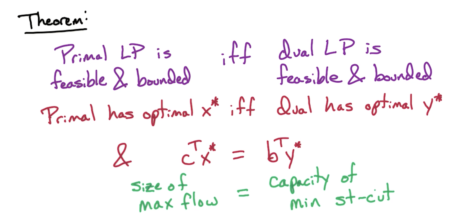
# Strong Duality
# Max-SAT Approximation
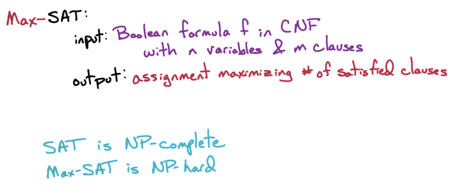
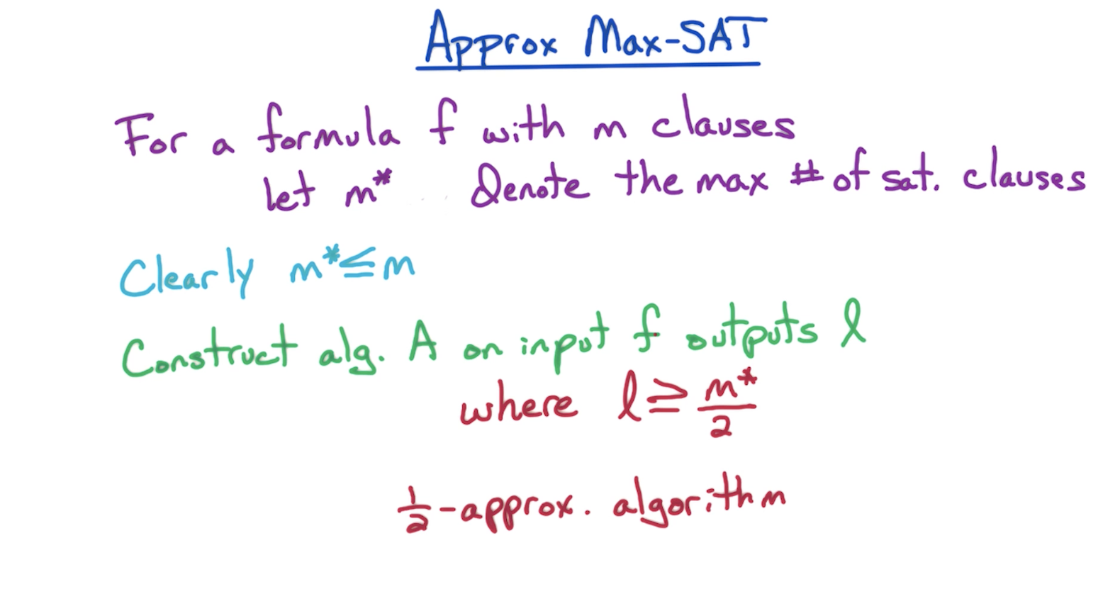
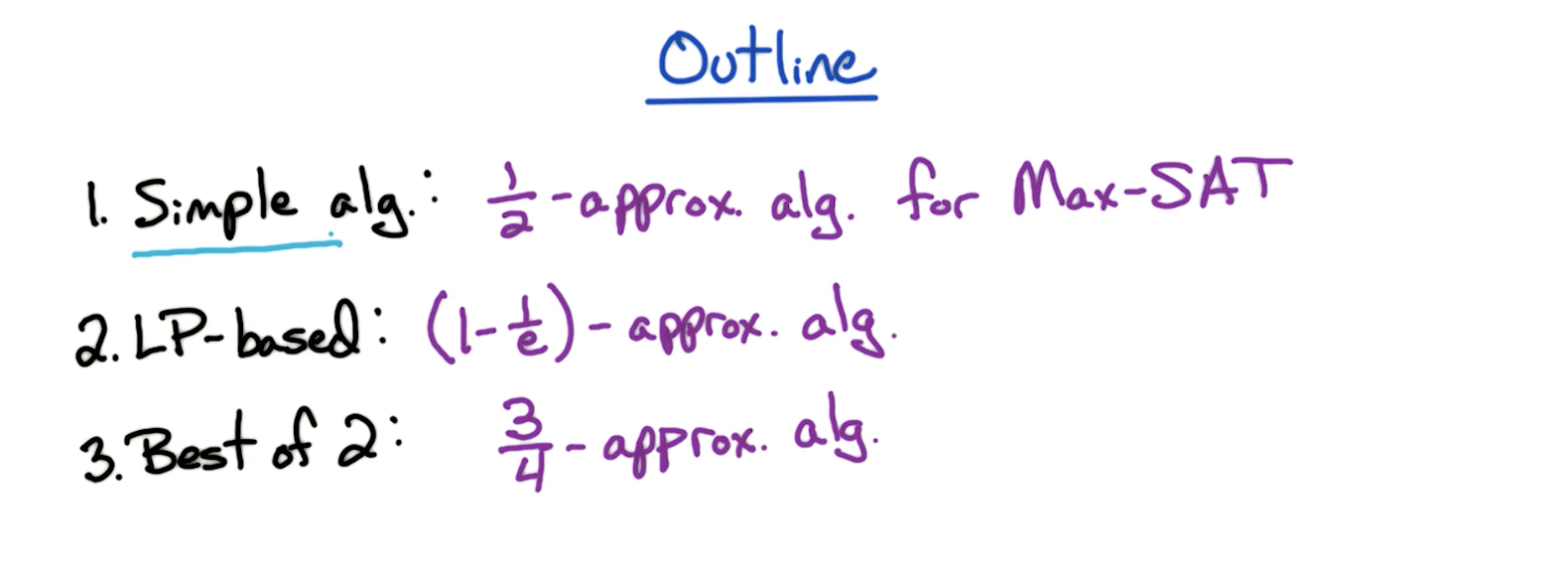
# Outline
# MAX-SAT: Simple scheme
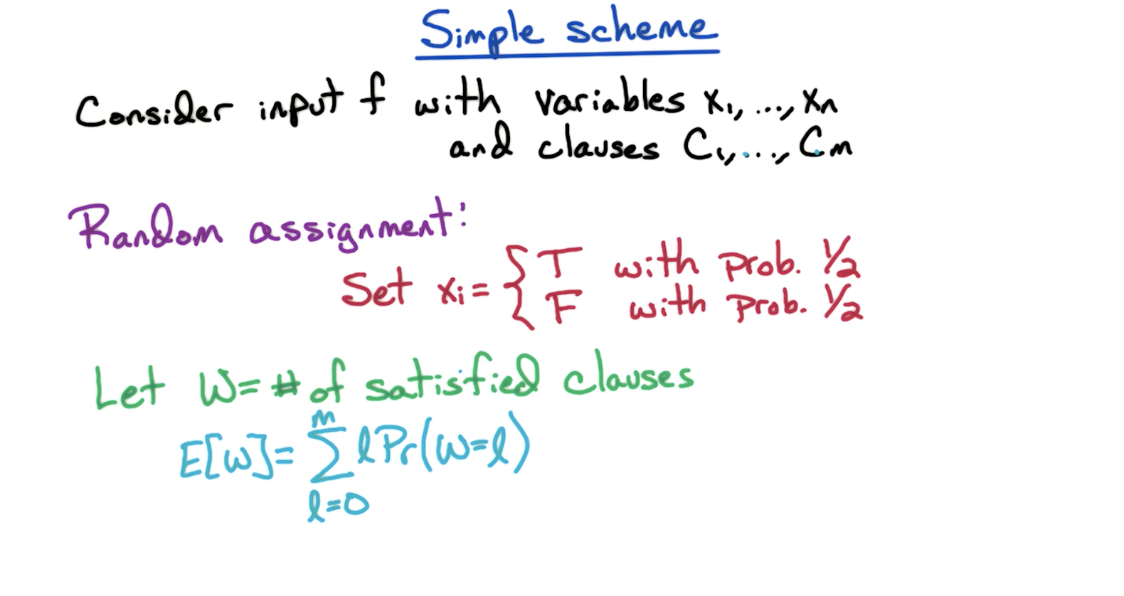
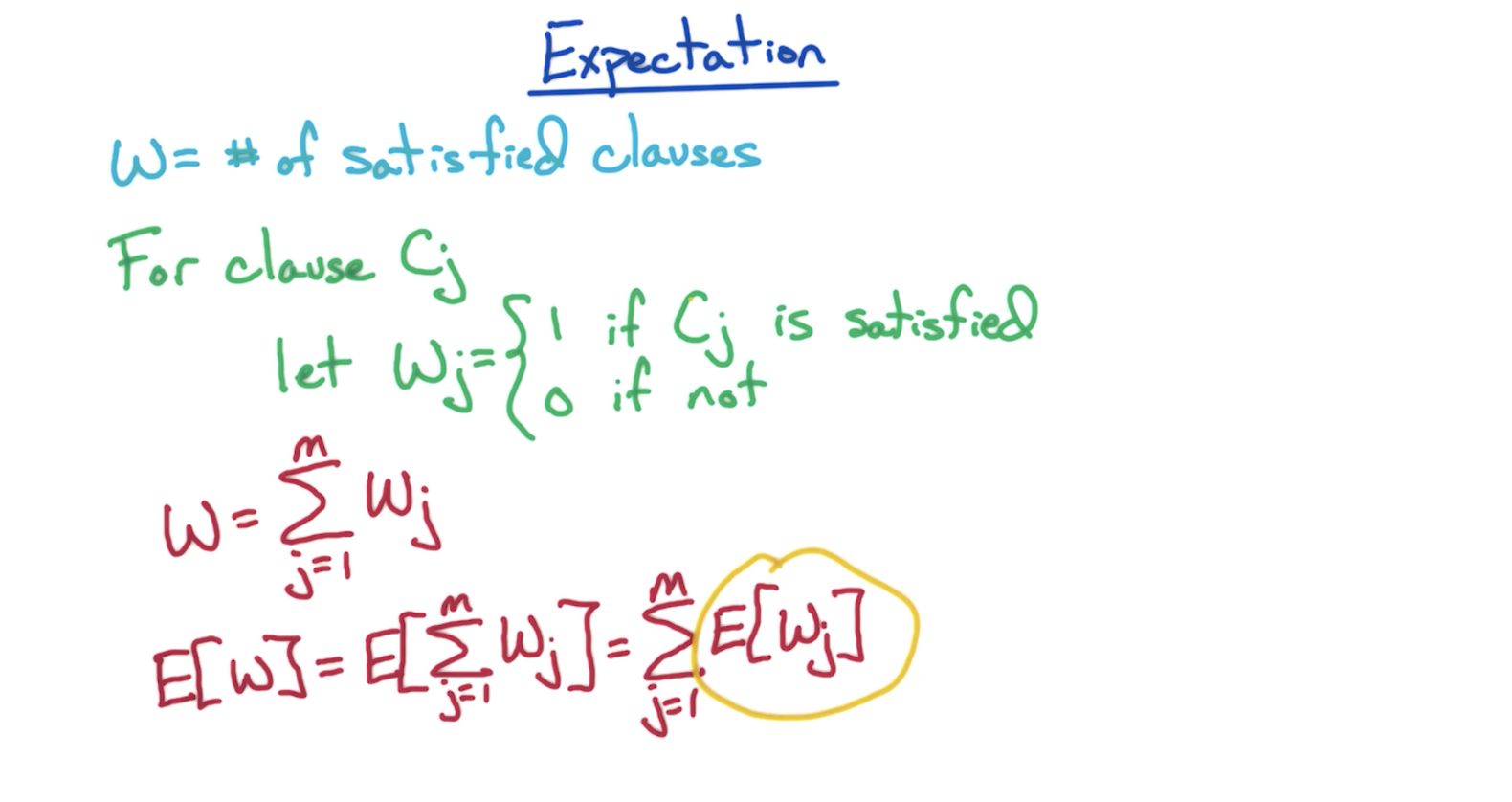
# Expectation
# Analysis
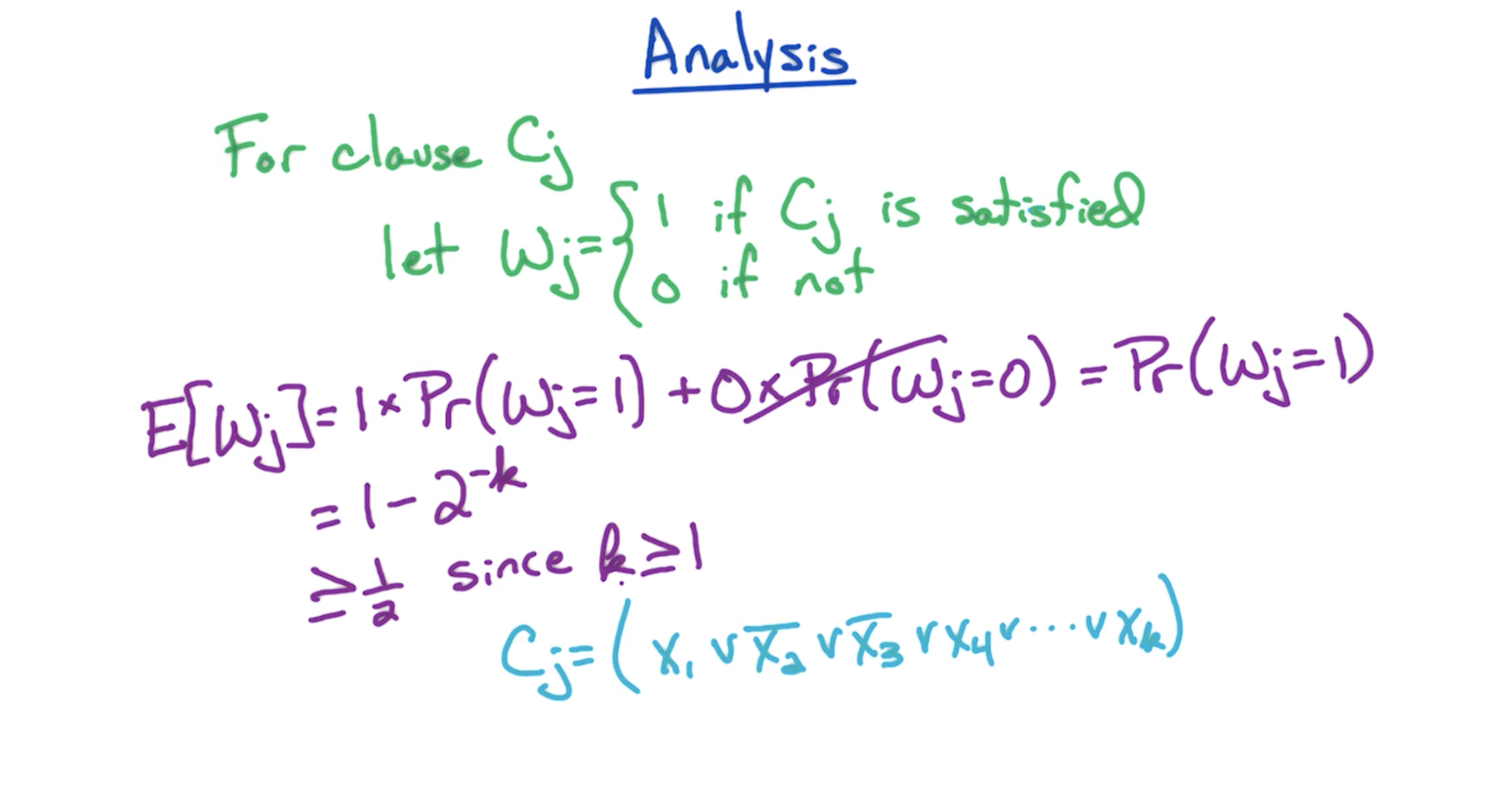
There is exactly one situation that
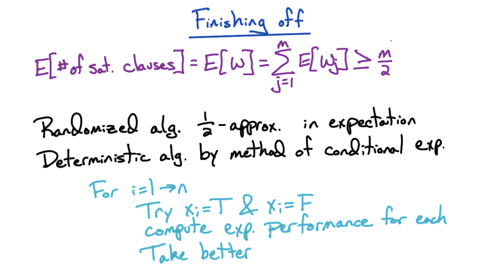
In the deterministic alg part described above, for each variable, we try two combos (T and F), while setting all other variables to random T/F. And we compute expected performance for each and take the better one. It is guaranteed to result in m/2 for the number of satisfied clauses.
# Ek-SAT
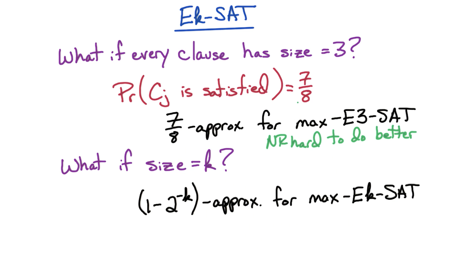
The intuition behind the 7/8 probability for
The challenge is with varying sized clauses where every clause does not have uniform number of clauses
# Integer Programming
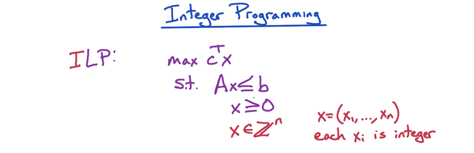
The difference of ILP compared to regular LP is that we have an additional condition where we only consider the integers in the feasible region as potential candidates for a solution. So instead of considering any real number in the entire feasible region, we place a grid in the feasible region that has the integer points, and we pick the best out of it.
On the surface, this can make ILP seem like a simpler computation but it isn't. LP had a property that there always is a vertex of the feasible region which is an optimal point maximizing the objective function. We no longer have such a property for ILP.
That's why :
- ILP is np-hard
# Max-SAT: ILP
Take NP-Hard problem
- Reduce to ILP
- Relax to LP & Solve
- Randomized round
# MAX-SAT: Alg Comparison

LP-based is better for k = 1 but simple scheme is better for k=3.
Therefore, for larger values of k, simple scheme is better. But for lower values of k, LP-based approach is at least as good, or even better.
Tip: Max in each row (best of the two schemes) >= 3/4
# MAX-SAT: Best of 2 Alg
Below is an algorithm that can get the best of the 2 algorithms.
Given f:
- Run simple algorithm - get m1
- Run LP scheme - get m2
- Take better of 2
And we can get
← NP