Useful Reads

Great visulization to understand Ford-Fulkerson

The lectures made much more sense after watching the above video

Algorithms

• Ford-Fulkerson
• Edmonds-Karp

Max Flow Problem

Input

The input to the Max-Flow problem is a Flow Network. A flow network is a directed graph G = (V, E) where vertex s is the source vertex and t is the sink vertex.

For each in E, a positive capacity is given.

Computation

We need to compute flows for each edge in the flow network such that supply can be sent from vertex s to t while maximizing the amount sent without exceeding edge capacities. denotes the flow along an edge

The following constraints must be met:

• Capacity constraint: for all
• Conservation of flow: for all , flow-in to v = flow-out of v

Goal

Find a valid flow of maximum size:

size(f) = total flow sent = flow-out of s = flow-in to t

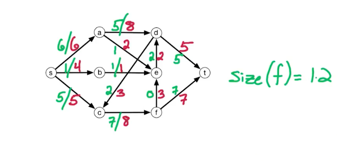
In the example above, the edges represent as values. The meet the capacity constraints described above. Also notice, for each vertex, in == out.

The size(f) is 12 since the two incoming to the sink vertex t add up to 12.

Concepts

• Having cycles is okay in a flow network. We might/might not use part of it depending on if it allows maximizing
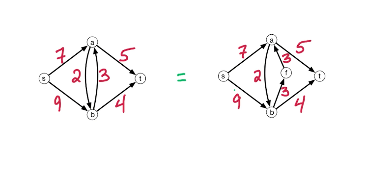
• Anti-parallel edges like shown below on the left are not okay for a flow network, as it makes it difficult while constructing a residual network later as it needs to add identical edges on the opposite direction. So we need to rewrite such edges like shown below on the right

Residual Network

Given the input of the flow network G = (V, E) with edges and weights as described in input above, and flow for :

is the residual network.

• if and then, add to with capacity

• if and then, add to with capacity (Backward Edge)

This entire concept is explained better in this video

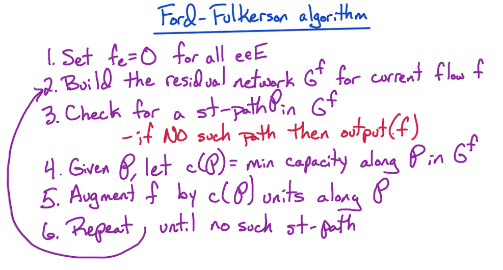
Ford-Fulkerson Algorithm

Running Time

Assume all capacities are integers, then flow increases by >= 1 unit per round.

Let C = size of max flow, then <= C rounds exist.

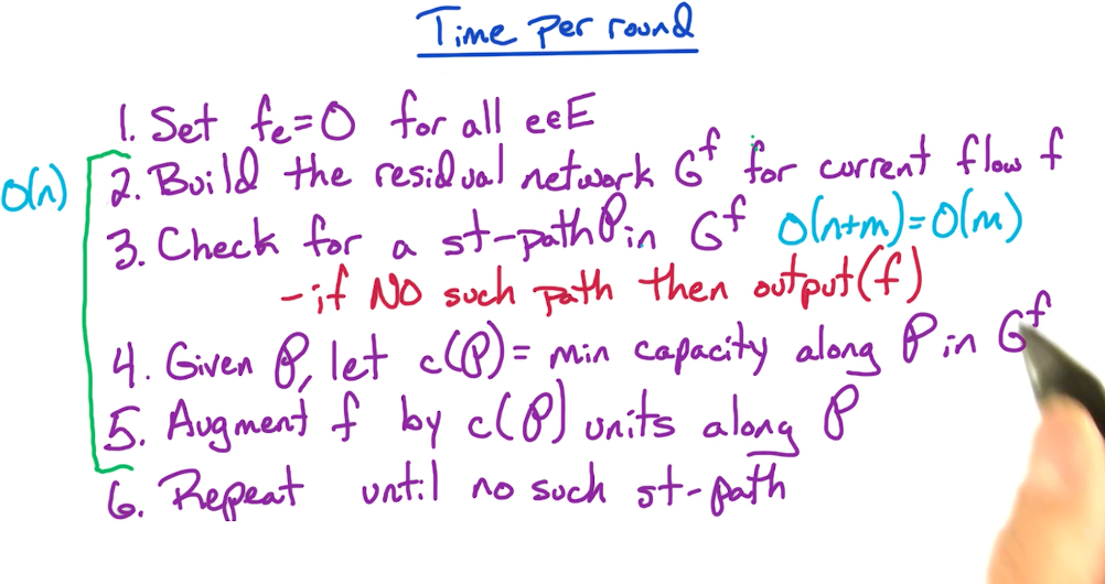
Since each round requires O(m) time, the total runtime is O(mC)

However, this assumes that the capacities are integer values and the running time depends on the size of the max flow. Therefore, it is said that the run-time is pseudo-polynomial, similar to that of Knapsack where the size decides the runtime. To address this, we have other algorithm like Edmonds-Karp.

Verifying max-flow

• Build a residual graph O(n+m)
• Check path from in residual graph
  • Run DFS from s to see if a path exists to t.
  • If no path exists in the residual graph from s -> t, then this is the max flow.

Min-cut Problem

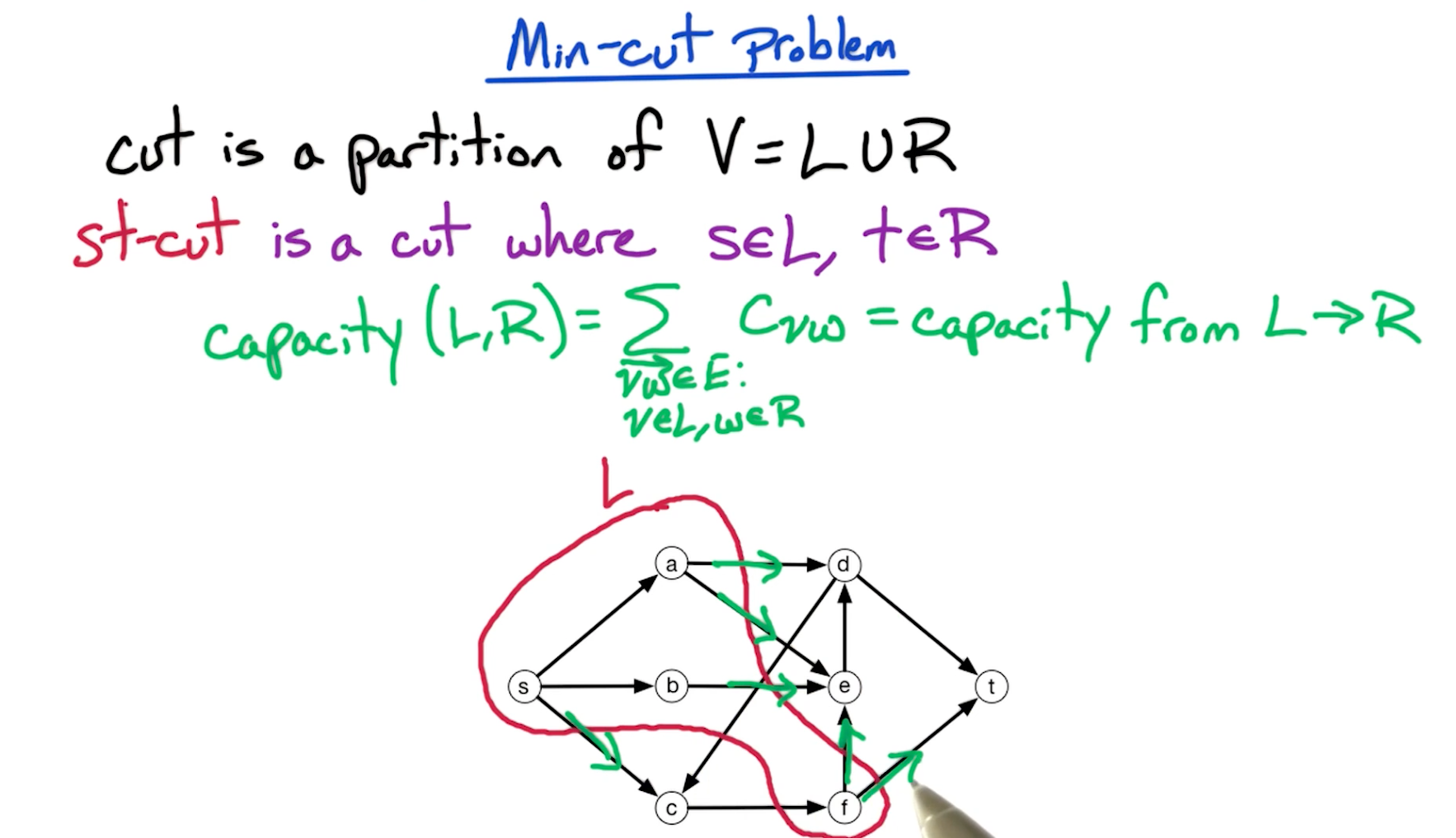
• Note that the vertices do not have to be connected for them to belong to either L or R. For e.g. vertex f is not connected to a or b in the L cut above.

• We only care about the outgoing edges from the cut highlighted in green.

Input/Output

Input: Flow Network

Output: st-cut (L, R) with min capacity.

By a st-cut with min capacity, we mean a cut such that it yields the minimum sum of capacities of all outgoing edges from L cut towards R cut. The example cut shown above doesn't get the minimum capacity though, it's just one of the example cuts.

Max-flow Min-cut Theorem

Explained well in this video after 17:30

Thereom:

To prove this theorem, we are going to prove two relations.

If both the above relations are proven, then that infers

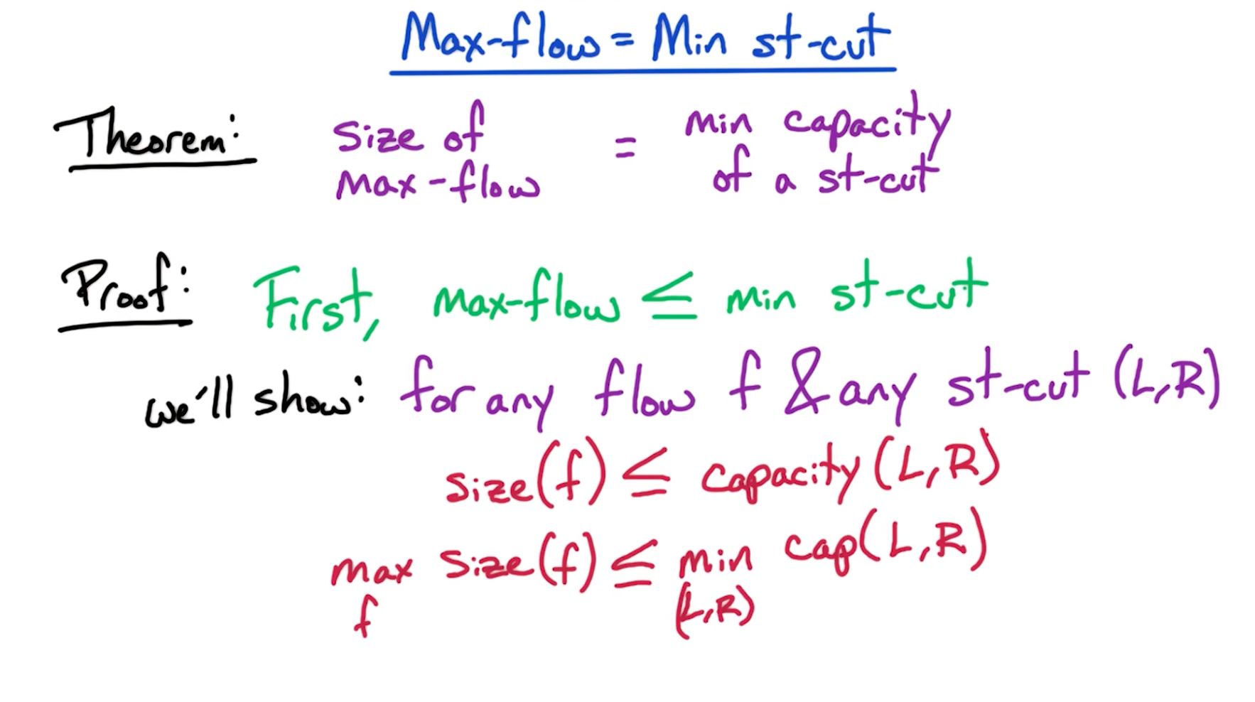
To prove the first equality below,

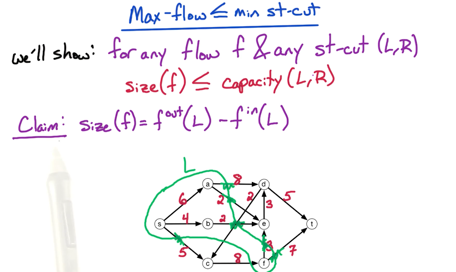
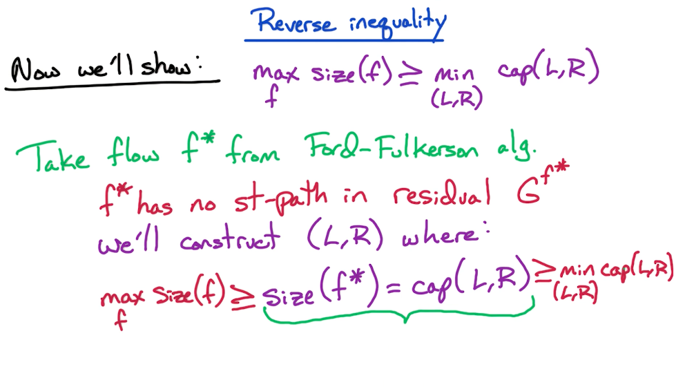
We get the , we simply sum the capacities of outgoing edges from L to R. In the following graph case, that equals to 27 (8+2+2+5+3+7) (or 29?). And the idea is to show that the size of flow is less than or equal to this capacity.

To prove the second equality below,

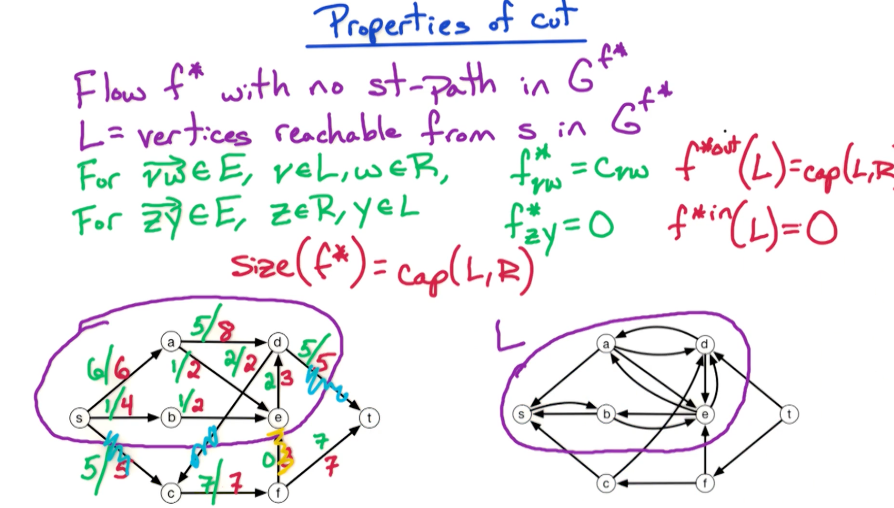
Properties of Cut

After the flow is filled (left graph), we can create a residual graph of forward and backward edges (right graph). We can construct this using the logic below.

• backward edge present: if positive flow exists in an edge
• forward edge present: if capacity is leftover in an edge

In short, fully capacitated edges are only one-way.

Then, L is the set of vertices reachable from s in the residual graph.

And R contains the remaining edges.

Tip: All the edges leaving L have to be unidrectional (and hence fully capacitated), otherwise, they'd have a way back to L and if that's the case, they'd have to be included in L.

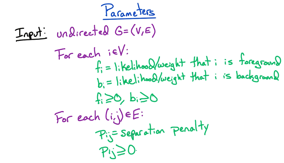
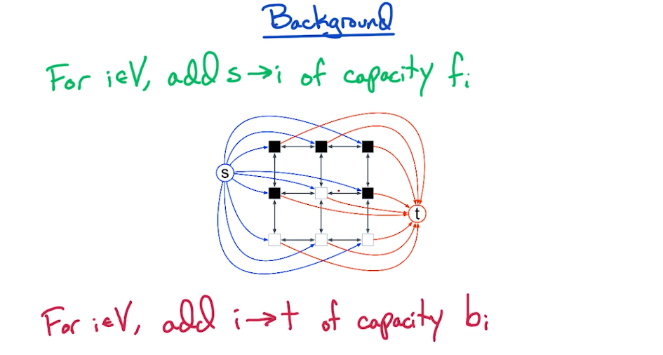
Image Segmentation

Parameters

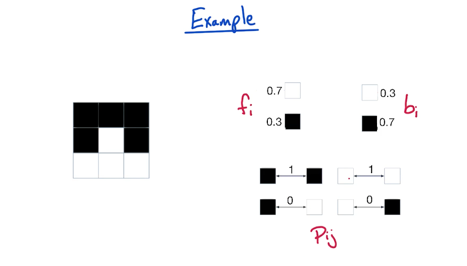
Example

Partition

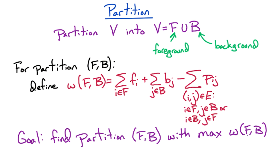
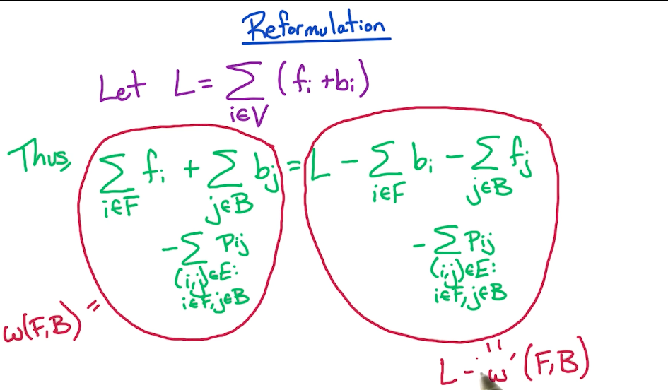
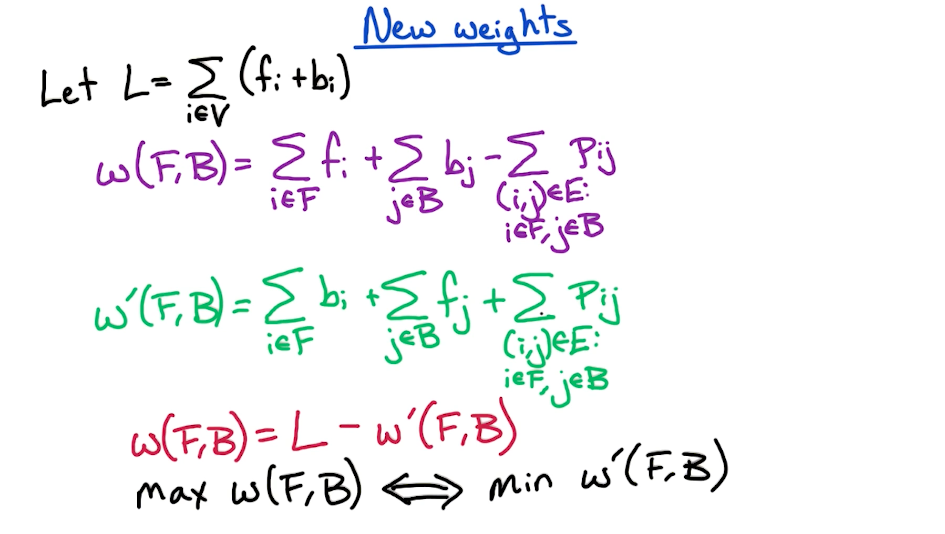
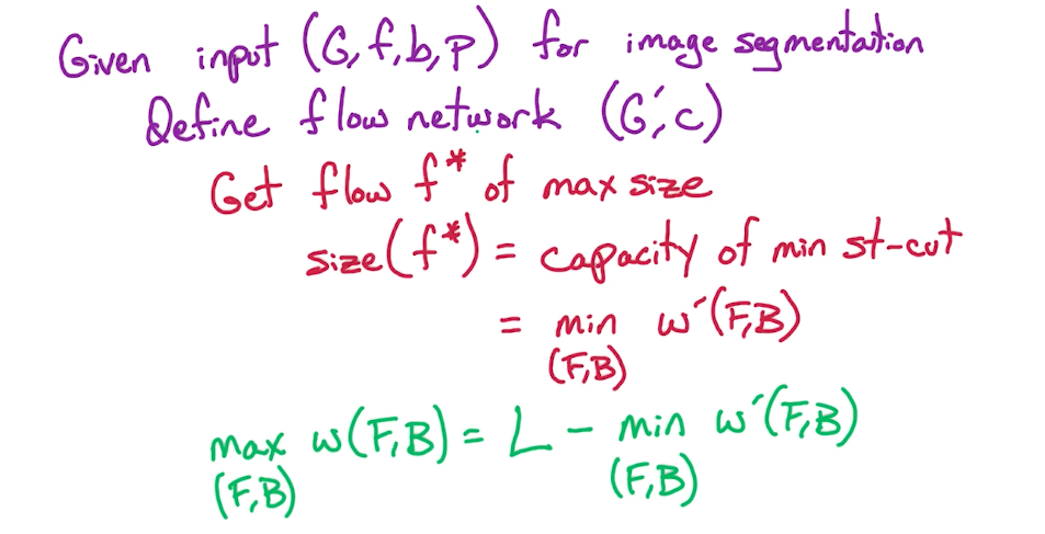
We have to reformulate this to a min-cut problem, for which we need to get rid of the negative sign in the expression.

Reformulation

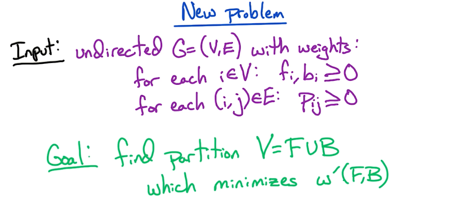
New Problem

Foreground and Background

Cuts

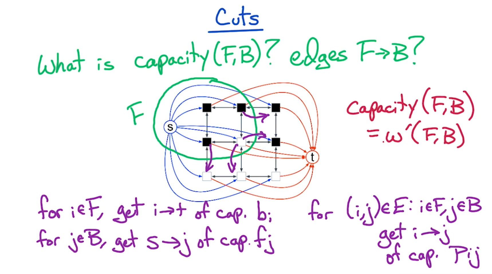
Solution

Generalization / with Demands

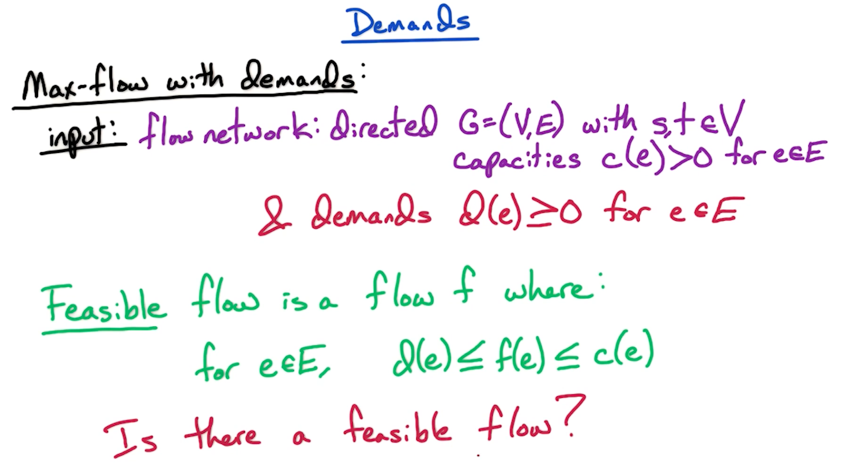
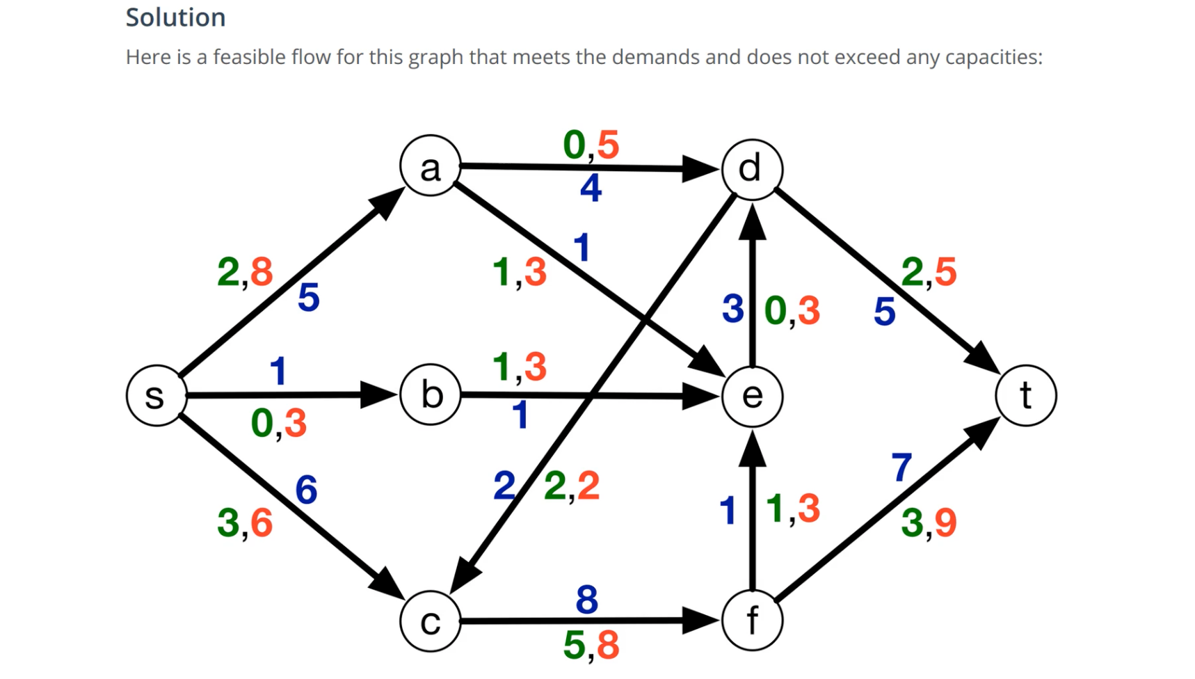
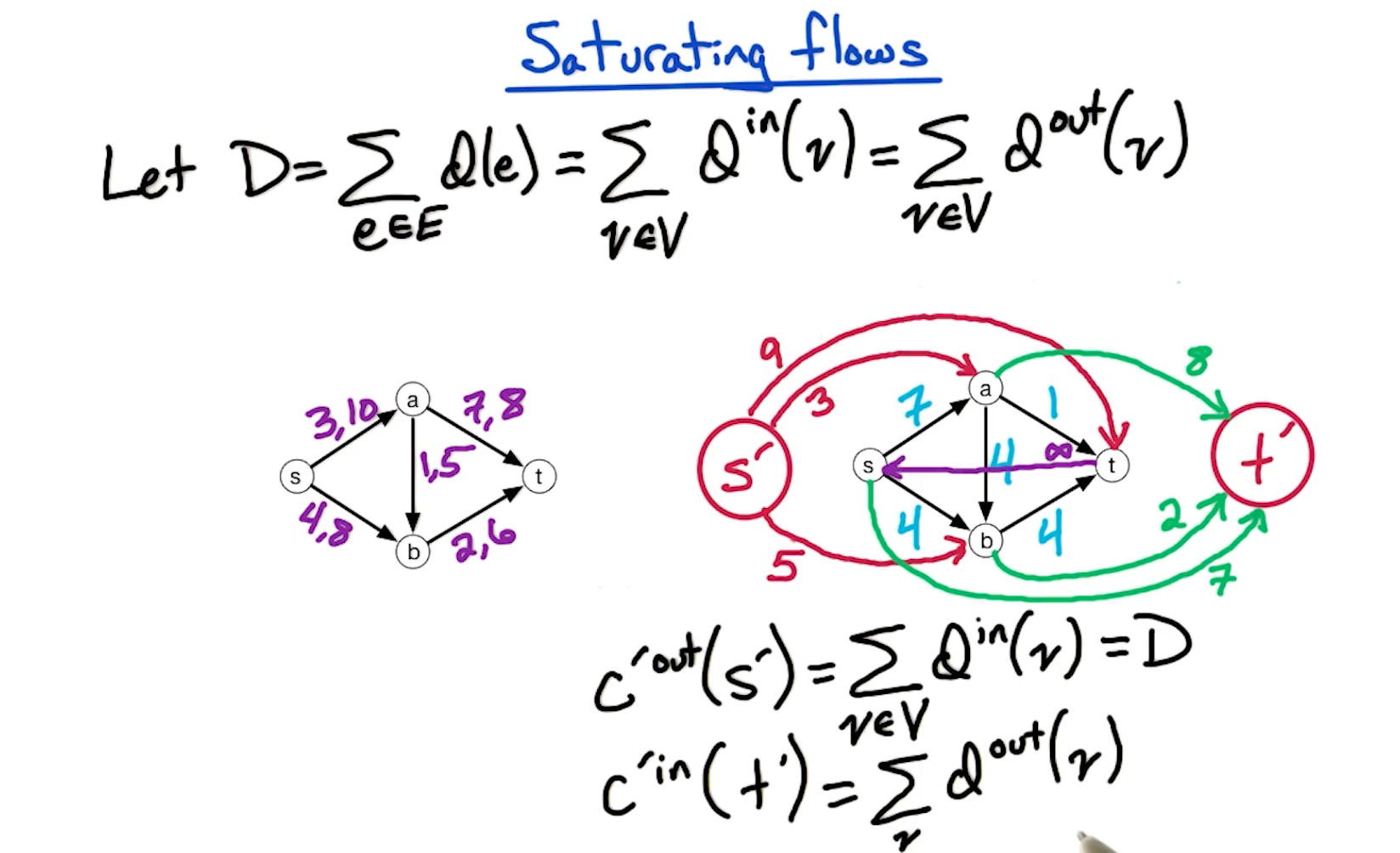
In the below example, the blue values are the flow values which is derived from the demand and capacity given in the format (demand, capacity) in each edge.

Tip: The idea is, in each edge, the flow has to meet at least the demand, and at most the capacity.

Reduction

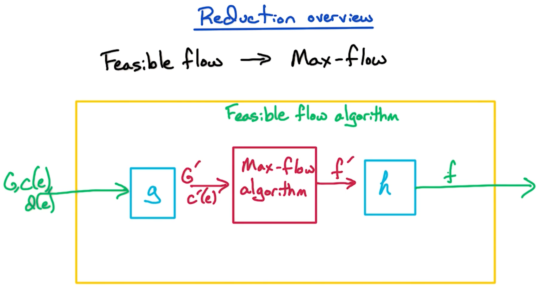
The general idea is taking the input to the feasible flow problem (graph $G$, capacities , demands ), and converting them to input for max flow problem (graph , capacities with a transformation function g. Then we run the max-flow black-box algorithm with these transformed inputs and generate the output. The output then again needs to be transformed to a feasible flow output using the h function.

Haven't been able to figure out the h part.

Following is the general algorithm for a g function that is supposed to construct from $G$

• Take the original set of vertices
• For each , add $e$ to with
• Add two additional vertices and
• For , add edge with
• For , add edge with
• Add edge with

Upon following these steps, we form a 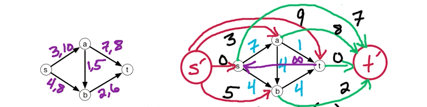that looks like below

Now we run max flow on the generated . When we complete running max-flow, we have to transform the output of max-flow to a feasible flow using function h. When flow in has a saturating flow, we can confirm that the original $G$ has a feasible flow. More on this below in the saturating flows section.

Some additional tips:

Intuition for original edges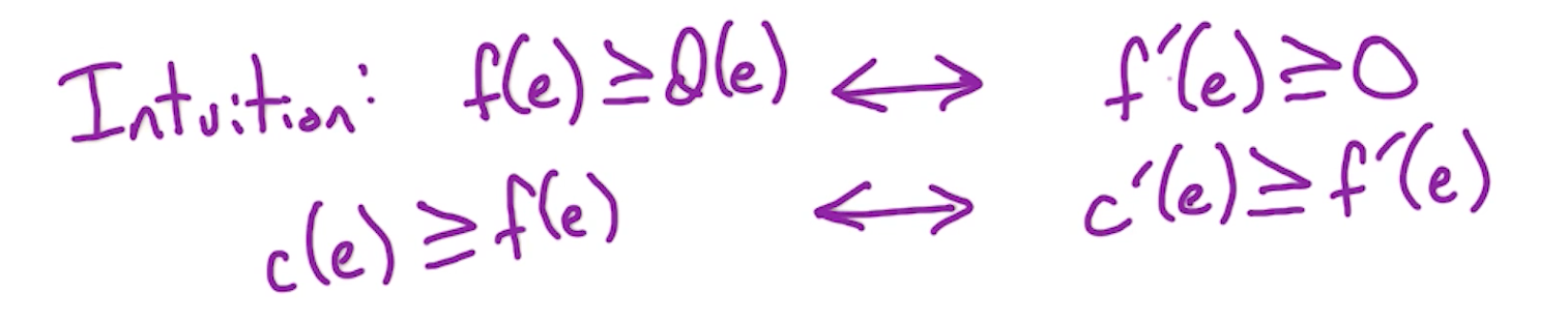

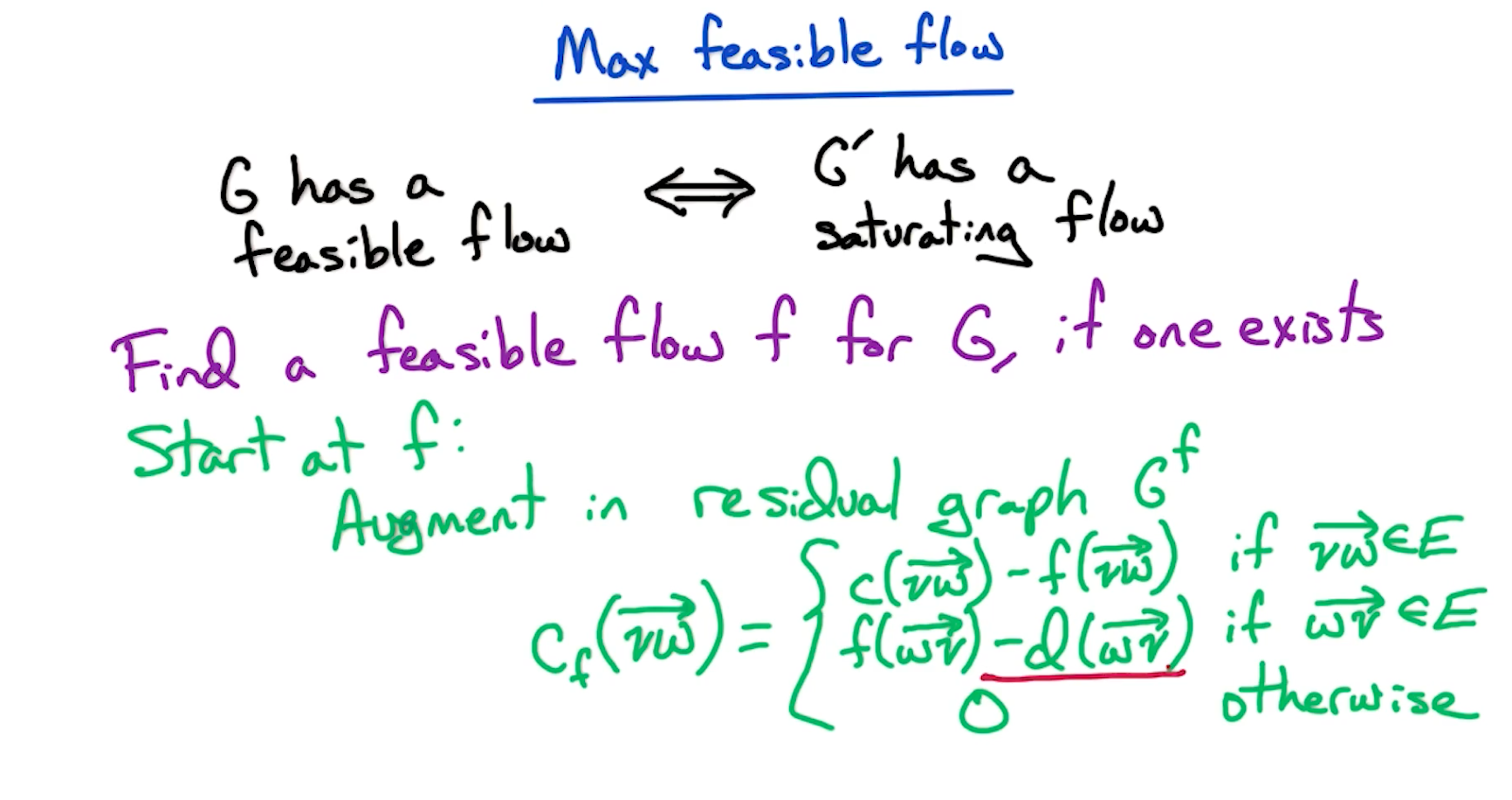
Saturating Flows

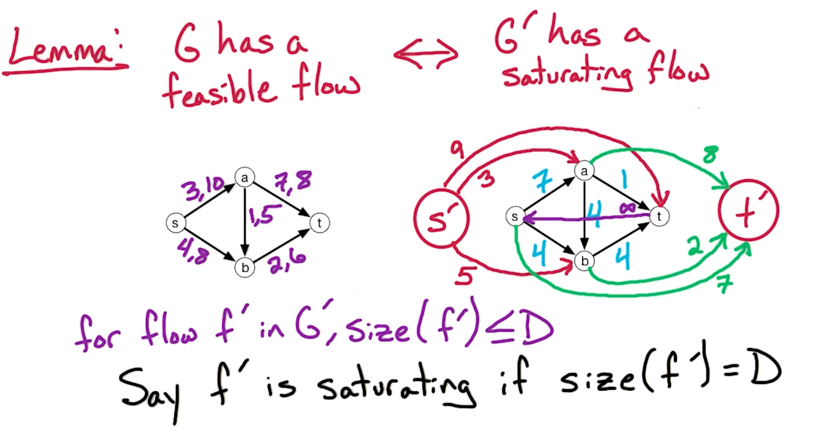
How to show a saturating flow is feasible?

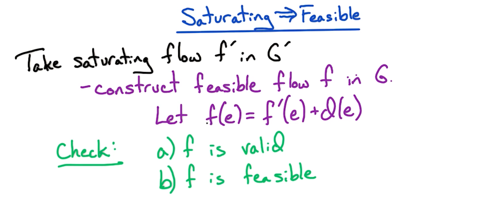
• To show f is valid, we need to show
  • flow-in = flow-out for all vertices in G created above,
  • flow along an edge is not higher than the capacity
• To show f is feasible, we need to show
  • all the demand consraints are satisfied

How to show a feasible flow is saturating?

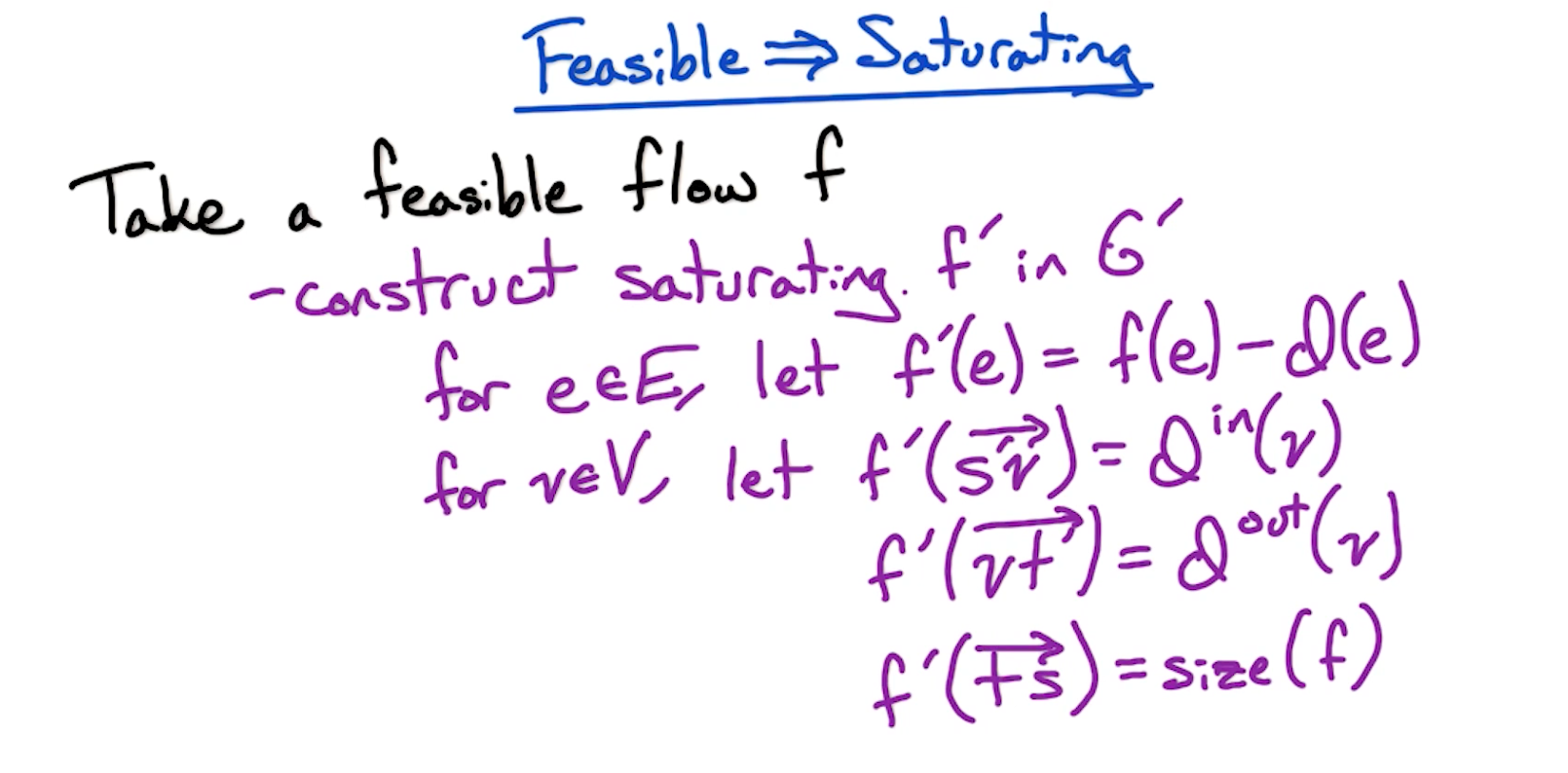
Not sure of the following

• To show is valid, we need to show
  • flow-in = flow-out for all vertices in G created above,
  • flow along an edge is not higher than the capacity
• To show is saturating, we need to show ...

Max Feasible Flow

Edmonds Karp Algorithm

• Identical to Ford-Fulkerson except a few differences
• Ford-Fulkerson finds augmenting paths using DFS or BFS, Edmonds-Karps uses BFS.
• Ford-fulkerson's time complexity is where C is size of max flow. The time complexity of Edmonds-Karp is
• Ford-fulkerson assumes integer capacities whereas Edmonds make no such assumptions

BFS Properties

Lemma: In every round, residual graph changes (>=1 edge deleted). For every edge e, e is deleted and reinserted later times. Since m edges, total rounds

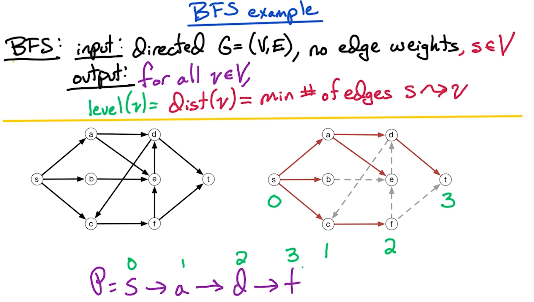
In the above example, the numbers correspond to the level of the graph. Since BFS expands equally in all directions and explores all unvisited nodes at a level before moving to the next level, this illustration is helpful to understand.

Claim: For every , level(z) does not decrease. It can increase, or stay the same, but not decrease.

Claim: If we delete from residual graph and later add , then increases by

Residual graph change

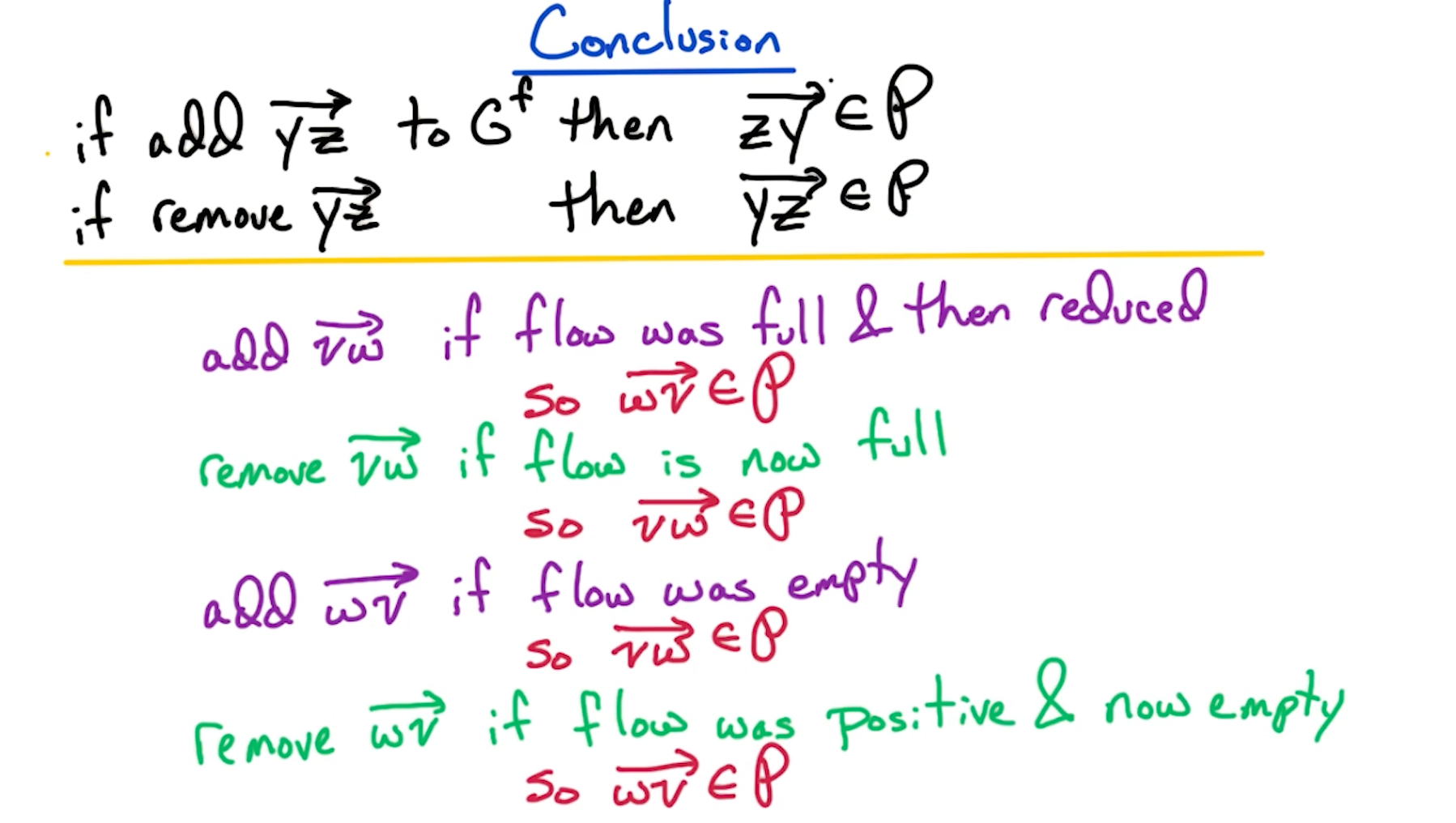
To get an intuitive sense for this, first understand what a "residual" graph means. A residual graph is tracking the residue or left over capacity. So:

• If a forward edge exists along an edge, it means there is capacity left along that edge.
• If ONLY forward edge exists, that means all of the capacity is remaining along that edge.
• If a backward edge exists, it means some of the capacity is used by flow.
• If ONLY backward edge exists, that means all of the capacity is used by the flow, and no leftover capacity exists.

Now based on this understanding, re-evaluate the above picture and it might explain when a forward or backward edge should be added or removed.