Fourier Transform

$f(t) = Acos(n\omega t)$

where

• A stands for amplitude,
• w for frequency.
• t determines how long the signal is
• determines how frequent the signal is where n is value and omega is just omega
• and A determines how high the frequency is

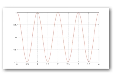
In the following graph,

• t = 4 (y-axis)
• A = 1 (a-axis)
• n = 2 (each time interval (t=1) gets two signals as you can see)

If you add multiple cosines f(1), f(2)... you end up with an impulse function with spikes at regular intervals

Definition

Periodic Function can be written as a weighted sum of sines and cosines of different frequencies.

A fourier transforms where the unit is time into a where is frequency. In other word, frequency spectrum of function f. So the function is no longer looked at in timesteps in seconds but in frequency spectrum of freq/spec, hertz.

• This transformation has to be a reversible operation.
• For every from 0 to infinity, holds the amplitude A and phase of a sine function

$f(t) = Acos(n\omega t + \phi)$

As frequency increase, the amplitude goes down

Frequency spectrum

Blending

Optical Window Size for Cross Fading

• To avoid seams: Window = size of largest prominent feature
• To avoid ghosting: Window <= 2x size of smallest prominent feature

Using fourier domain to come up with optimal window sizing

• Largest frequency <= 2x size of smallest frequency
• Image frequency content should occupy one octave (power of 2 )

Feathering

Think of blurring out the edges in the masks so the jump isn't steep

Pyramid Representation

You move a gaussian kernel over an image to get its smaller version, and if you do this recursively, you'll get a series of images, which when stacked up make it a pyramid view. The top ones (smallest ones) give you a coarse represntation, whereas the bottom of the pyramid, the original high def ones give you a fine representation

Here means it is g(0) expanded 1 times (or g(0) achieved by expanding its next smaller image)

Expand is inverse of reduce, as it seeks to add new values in between known ones. Obviously, expand will have some errors for that very reason.

Cuts

Blend might not always be the best fit to merge image since it relies on taking some combination of corresponding pixels in the two pictures based on a weight. Ghosting might be a common issue while blending.

With cutting, you select pixel from one image or the other by figuring out the points of cuts.

Seam Carving seems awesome (to stretch and squeeze images)

Check it out yo!

Low Pass - High Pass Filters

• A filter that attenuates high frequencies while passing low frequencies is called low pass filter.

Low pass filters are usually used for smoothing.

• Whereas, a filter that do not affect high frequencies is called high pass filter.

High pass filters are usually used for sharpening.

Laplacian Pyramids

• “The Laplacian Pyramid as a Compact Image Code" (Burt and Adelson; 1983)
• “A Multiresolution Spline With Application to Image Mosaics” (Burt and Adelson; 1983)

You will notice convolution formula in there, which might seem strange, but it it is essentially the same as we have in the notes before. The only difference is instead of values like (i + m) now there is (2i+m) in REDUCE because we're taking strides of 2 to downsample the image to half

And likewise, instead of values like (i + m) now there is (i - m) / 2 because in EXPAND

This guy explains it well.

Instructions from A2 inline comments show another interesting way to implement this same thing without rewriting convolution. It involves an approach like the following

reduce_layer: pad -> convolve -> subsample by taking every alternate element in matrix

expand_layer: upsample by adding alternate rows/cols and filling them with zeros -> pad -> convolve

Features

Characteristics of Good Features

• Repeatability/Precision
• Saliency/matchability
• Compactness and efficiency
• Locality

Finding Corners

• Key property: In the region around a corner, image gradient has two or more dominant directions
• Corners are repeatable and distinctive

An image moment is a weighted average of image pixel intensities or can be a function of those intensities. And it is used to give properties at a point within an image. We will leverage here information gotten from derivates like and where they represent the intensities in X and Y directions respectively

Think of Eigenvalues like this

You condense a matrix to smaller values such that you can bring it back to its original form/scale it up by using a scalar value. That scalar value is the eigenvalue. If you look at the diagram above, if the eigenvalues scale both X and Y, you end up with something on top right, otherwise depending on which dimension they're scaling, you could end up with views like in the other three corners.

In the case above in the picture, you can get away without using eigenvalues if you have the second moment matrix (M), for which you'll just be taking derivates of image intensities as shown in the preceeding image.

Look at 3Blue1Browns Video on Eigenvalues to understand this better

Harris Detection Algorithm

How to apply

1. Compute horizontal and vertical derivates of the image i.e. compute Gaussian derivates at each pixel i.e. convolve with derivate of Gaussians
2. Compute second moment matrix M in a Guassian window around each pixel
3. Compute corner response function R using the M gathered above
4. Threshold R
5. Find local maxima of response function (non-maximum supression)

Better visuals here starting Harris Detector Step by Step Video

• Step 3 highlights the corners.
• With 4, we threshold those highlights to only bring out highlights above a certain threshold, so we get the brightest areas that are most likely corners.
• With 5, we get dots such that we get the local maxima in each of the regions.

OR JUST APPLY cv2.cornerHarris lol

Properties of Harris Detector

• Rotation Invariant
  • Ellipses rotate, but shape (eigenvalues) remain same
  • corner response R is invariant
• Intensity Invariant
  • Partial invariance to additive and multiplicative intensity changes (threshold issue for multiplicative)
  • this is because we rely on gradients/derivates
  • only image derivates are used
• Not Scale Invariant by default
  • Dependent on window size
  • You can make it scale invariant by using the approach outlined in pic below.
  • use pyramids (or frequency domain)

Choosing Corresponding Circles

• Pick a region that is "scale invariant"
• This region should not be affected by the size but will be the same for "corresponding regions"
• For e.g. average intensity. For corresponding regions (even of different size), it will be the same
  • Compute a scale invariant function over different size neigborhood

Scale Invariant Detectors

Invariant detectors are great because they help us detect invariant local features. Basically, image content is transformed into local feature coordinates that are invariant to translation, rotation, scale, and other imaging parameters

So use pyramid to find maximum values (remember edge detection?) - then eliminate "edges" and pick only corners

Harris-Laplacian

Find Local maximum of

• Harris corner detector in space ( image coordinates)
• Laplacian in scale

Can find features despite the zooming of images

SIFT (Scale-Invariant Feature Transform)

Find local maximum of

• Difference in Gaussians (DoG) in space and scale
• DoG is simply a pyramid of the difference of Gaussians within each octave

Or in other words, do the following two in sift:

Orientation Assignment - Computes best orientations for each keypoint region

Keypoint Description - Uses local image gradients at selected scale and rotation to describe each keypoint region