# Stages
Illumination -> Optics -> Sensors -> Processing -> Display -> User
All about converting rays of light to pixels.
# Surfaces
- specular (mirror)
- diffuse (matte)
# Dual Photography
Amazing Stanford Research on Dual Photography
# Digital Image Representation
- A grayscale image's pixel can have values in the range 0-255, then you would need 8 bits to represent it cause each binary place has two possible states and
- You can represent grayscale images in 2D matrices but RGB color images would be 3D, because they also have an additional color dimension. To store tho, you would need
possible states (8 bit for each channel) which makes it a 24 bit image. - Images can be represented in discrete values or function
# Cool Analytical Things
- Height Map is cool, Histogram sampling intensities is cool
- Image based, Region based, Channel(RGB) based sampling of intensities to generate histograms
# Point Process
- Alpha Blending: Multiplying an image with a value between 0-1, that makes the image a little transparent since it is making the values in the matrix smaller. If you merge two-three images by doing this to all, you blend them interestingly by making some transparent - remember the einstein, darwin example.
# Arithmetic Blend Modes
Formula using 0-1 scale instead of 0-255)
- Divide (Brightens photos)
- Addition (too many whites)
- Subtract (too many blacks)
- Difference (subtract with scaling)
- Darken (min(a, b) for RGB)
- Lighten (max(a, b) for RGB)
- Multiply (
, Darker) - Screen (Basically opposite of Multiply,
, Brighter) - Overlay (Combines Multiply & Screen. if
, then . Otherwise, ) - Dodge & Burn (Dodge builds on screen mode, burn builds on multiply)
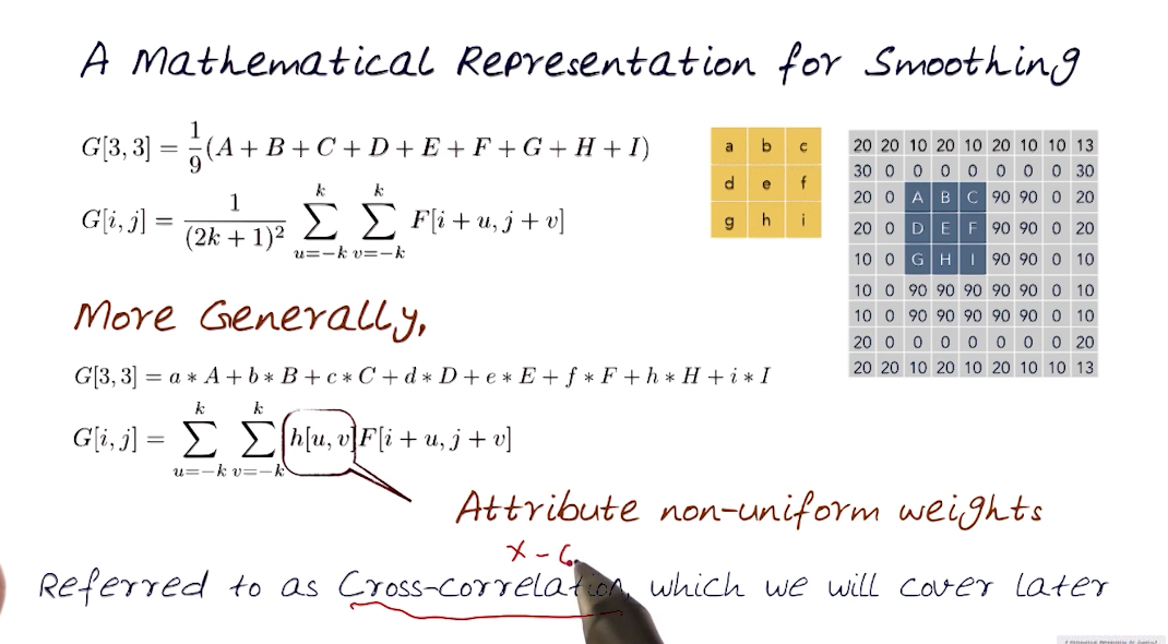
# Smoothing
- Averaging the neighboring values - moving left to right, by going over a 3x3 grid applying the filter/kernel. Can give more weights to nearby ones and less weight to farther ones.
- For the edge pixels, you can't have enough neigbors, so you'd have to pad additional row/columns depending on the size of the kernel. You can wrap around, copy edge or reflect across edge.
- Window size is 2k + 1 = 3x3. Where k is the neighborhood size.
# Box Filtering / Averaging Filtering
- Makes an image blurry.
- Using a large, something like 21*21 kernel will degrade the image on the edges due to extra 10 padding added.
# Median Filtering
- Median Filter has no kernel, cause you are basically analyzing the image and updating values.
- Nonlinear operation that reduces noise but preserves edges and sharp lines.
- Great for noise removals like salt and pepper noise
# Gaussian Filter
- Just like a gaussian, the central regions get more weights (imagine in 3d valley view).
- A gaussian kernel has to be generated first specifying the kernel size and sigma value using something like
cv2.getGaussianKernel - Increasing the kernel size helps smoothen the image. Going from 3 to five. Since it weighs in more of its neighbor to add the smoothness.
- The higher the sigma/variance used to generate the kernel, the more blurry the resulting image is.
# Sharpening Filter
- Raising the sigma made the image sharper.
- Also raising the beta value seemed to help, probably because of allowing gaussian to play an important role
# Signal Processing
# Cross-correlation Method
- In signal processing, cross-correlation is a measure of similarity of two waveforms as a function of a time-lag applied to one of them.
- Also known as a sliding dot product or sliding inner product.
- Filtering an image means replacing each pixel with a linear combination of its neighbors. the kernel servers as the weights in the linear combination. Just adding up the products of kernel element at x with image's element at x in the current sliding window and normalizing it.
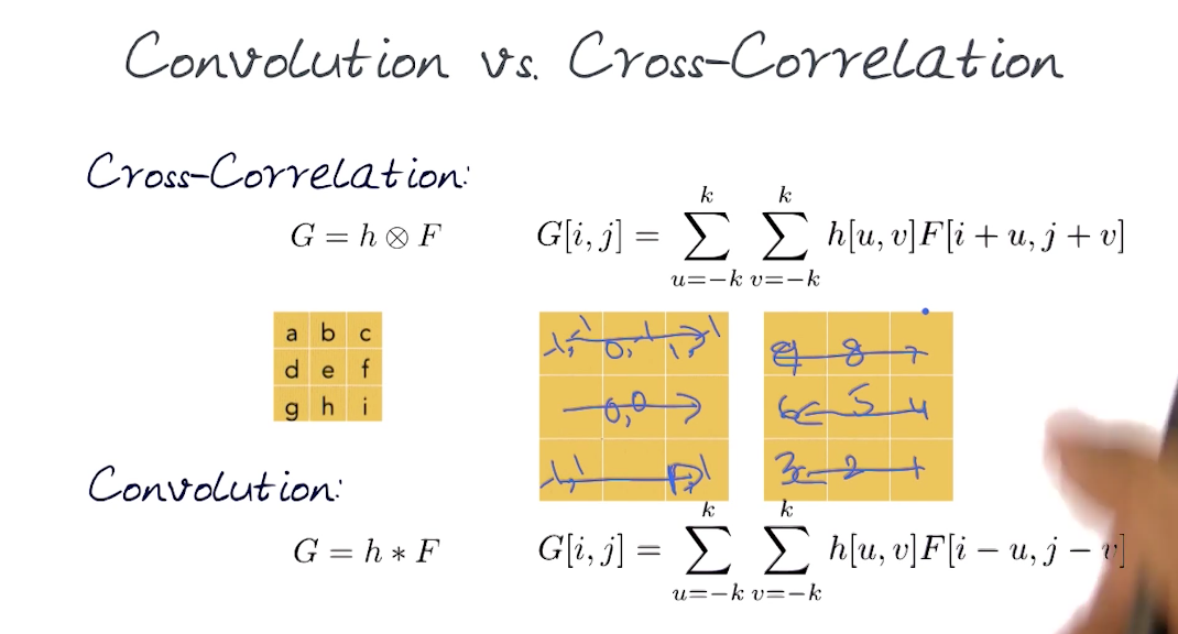
# Convolution Method
- Example demonstrated by showing Impulse function (peak(1) in middle of the image while leaving everything else dark(0)) passed through a kernel gives you a result that is inverted across both x and y axis.
- Using this you can say the convolution method gives the area of overlap between the two functions (image function and kernel function) in the form of the amount that one of the original functions is translated.
Performing convolution is basically equals to flipping the original kernel bottom to top, then right to left and then applying cross-correlation.
# Convolution using Cross Correlation
- Flip the kernel in both dimensions
- Bottom to top
- Right to left
- Then apply cross correlation
In cross-correlation, the kernel is applied traversing the top left corner and ends at bottom right corner. In Convolution, the kernel is applied traversing from bottom right and ending in top left. This is why the above works. Flipping the kernel and then applying cross correlation is the same as just applying convolution. And vice versa.
The difference in the two summation formulas - cross correlation has a plus, and convolution has a negative. This is just to dictate the order of kernel traversal.
# Properties of Convolution
- Linear and shift invariants
- Behaves the same everywhere i.e. the value of the output depends on the pattern in the image neighborhood, and not the position of the neighborhood.
- Cummutative
- F * G = G * F
- Associative
- (F * G) * H = F * (G * H)
- F * Impulse kernel = F
- Separable
- If the filter is separable, convolve all rows, then colvolve all columns
# Edges / Gradients
# Edges
- Features are parts of image that encode it in a compact form
- Good features to match between images are the discontinuities
- Surface normal
- depth,
- surface color,
- illumination
- Edge encode change, therefore edges efficiently encode an image
- Edges appear as ridges in height maps
- Look for a neighborhood with strong signs of change
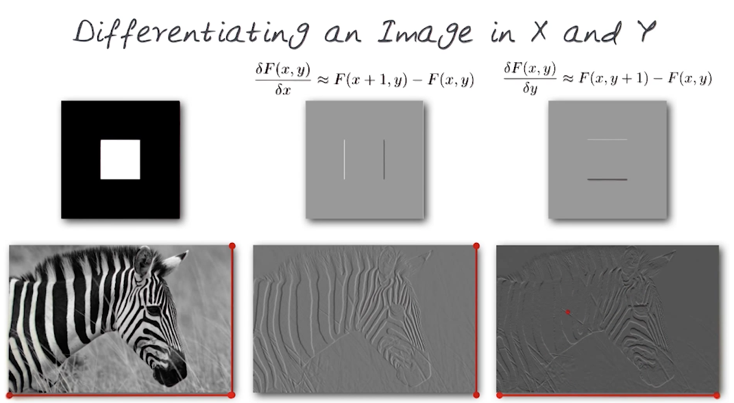
- An edge is where there is a rapid change in the image intensity function
# Questions to ask
- What is the size of the neighborhood? E.g. k=1
- What metrics represent a change? E.g. Difference threshold diff of 90
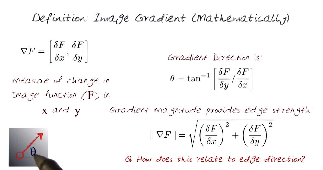
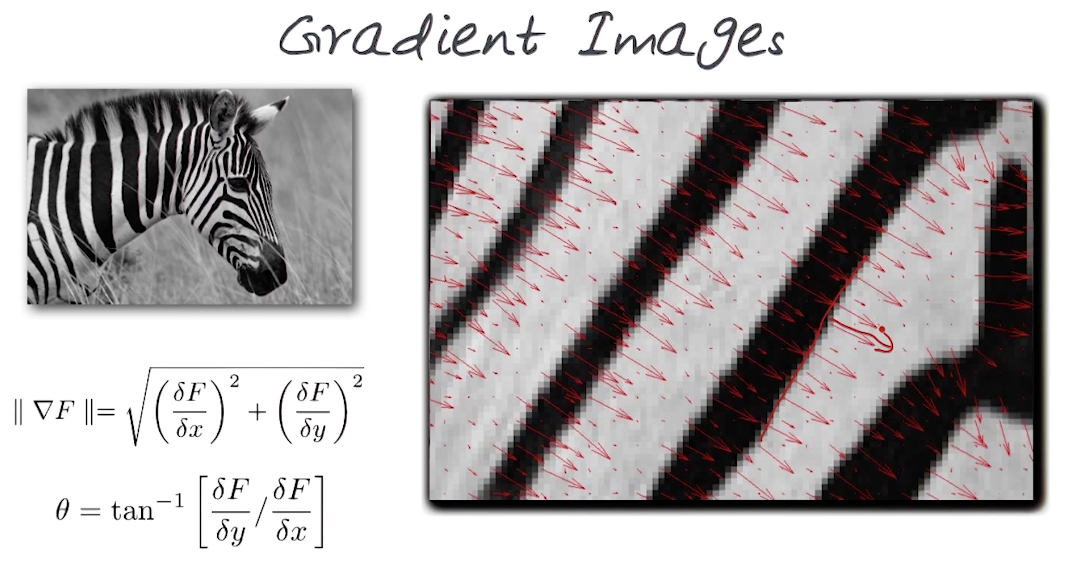
# Image Gradient Process
- Gradient of an image is the measure of change in image function
in x and y - Need an operation that when applied to image returns its derivatives
- Model these operators as kernels, which when applied, yields a new function that is the image gradient
- Then threshold this gradient function to select edge pixels.
# Edge Detection Steps
- smoothing: suppress noise, something like Gaussian filter
- compute gradient
- apply edge enhancement
- Edge localization (edges vs noise)
- Threshold, thin
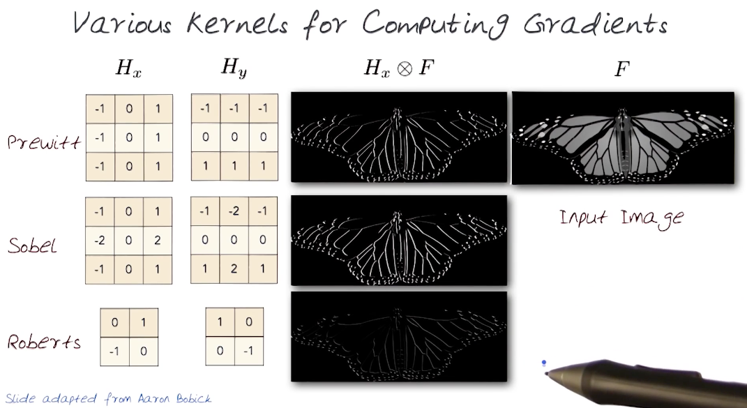
# Canny Edge Detector
- Filter image with derivate of Gaussian
- Find magnitude and orientation of gradient
- Non-maximum suppression
- Thin multi-pixel wide ridges down to single pixel width
- Linking and thresholding (hysteresis)
- Define two thresholds - low and high
- Use the high threshold to start edge curves and the low threshold to continue them