Motion Planning

Given: Map, starting location, goal location and cost function

Find: Minimum cost path

A Star key concept

• For every possible expansion, sum the G value (total number of steps that'll need to be taken to get to that expansion) with the Heuristic H (for.eg. euclidean distance to goal from that expansion)

$f = g + h(x,y)$

• Out of the possible expansions, pick the one with the lowest f value.
• In the A* search algorithm, if the heuristic function is admissible, A* is guaranteed to return a least-cost path from start to goal.

Dynamic Programming for Robot motion planning

With dynamic programming, you will be able to find best path from any given location instead of the one start position.

There is no bearing of the start position on this, since the policy is focused only on the goal state.

Value function conceptually

• Start from goal
• Take the optimal neighbor, and do: its value + cost it takes to get there from here
• do second step recursively until you cover the whole map so you have a value for each pos

PID Planning

Smoothing of path so the robot can move in a way that's more natural and avoid sharp turns

Smoothing algorithm

• Take the sequence of paths as x0...xn. Each x is technically an object representing a given position and not an x coordinate

• y series = x series

• While change is greater than tolerance, set change to zero, iterate once through all points and optimize using gradient descent while updating the change value, and compare change value with tolerance

  • Weighting & Smoothing:
  • change = change + abs( before applying above - after applying above)

If you set the weighting alpha to zero and don't change the start position and end position, you get a straight line path

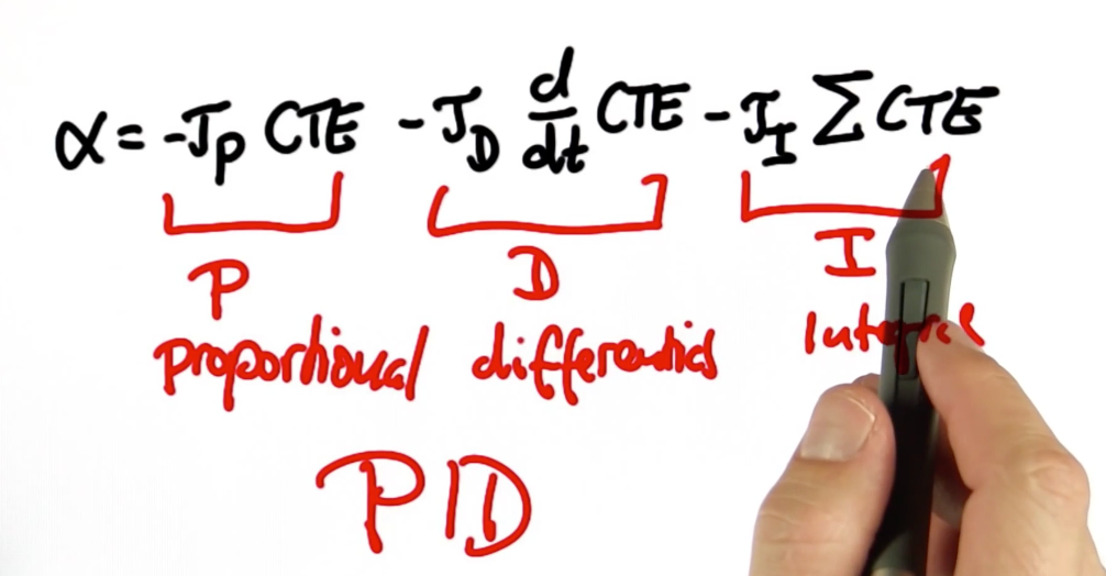
PID Control

P (Proportional control) steers it down, I (Integration) steers it up, and D (differential) dampens the oscillations and smoothens out. P - minimize error, I - Compensating drift and D - avoids overshoot.

Alpha is the steering angle, CTE is the cross track angle

Intuition behind hyperparameter tuning

• If you see a lot of ups and downs, tune up the to smoothen the signal
• If the signal stabilizes higher than the destination, drag it down by tuning up the
• If the signal needs to be brought up, tune up
• Don't forget about Integral unwinding when the direction of error changes (goes from positive to negative value or vice versa) because Integration values cummulative over time. Check the following things and if they return true temporarily turn off the integration switch (or you can also reset the integral value to zero)
  • PID control output is saturating (value from PID controller beyond the system's acceptable range)
  • The value of error and output from PID controller don't have the same sign

Twiddle

The Twiddle function discussed in the lectures is a hill climbing algorithm. The one big caveat is that it can get stuck in local maxima/minima depending on your error function. There are ways around it like to pre-prime the values to be discovered with values near the possible optima. Other ways to get around this are to use a different algorithm which is less prone to local maxima/minima like

• Stochastic Hill Climbing,
• Random Restart Hill Climbing,
• or some thing more advanced like Simulated Annealing.

Summary

• Finds continuous Path: Smoothing
• Finds optimal path: A*, Breadth First and dynamic programming
• Finds universal path: DP
• Finds local path: Smoothing

SLAM

Simultaneous Localization and Mapping

• Constructs a map as the robot moves and navigates the place

When mapping an environment with a mobile robot, uncertainty in robot motion forces us to also perform localization.

Graph SLAM Technique

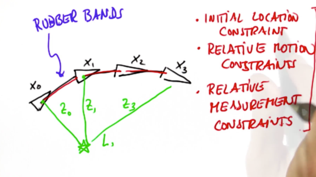
SLAM has continuous and discrete components. The continuous components are the locations of objects in the map and the robot's pose variables. The discrete components are the correspondence variables. From Probabilistic Robotics p. 310: SLAM problems possess a continuous and a discrete component. The continuous estimation problem pertains to the location of the objects in the map and the robot’s own pose variables. Objects may be landmarks in feature-based representation, or they might be object patches detected by range finders. The discrete nature has to do with correspondence: When an object is detected, a SLAM algorithm must reason about the relation of this object to previously detected objects. This reasoning is typically discrete: Either the object is the same as a previously detected one, or it is not.