Comparison with other techniques

Tracking Approach	Monte Carlo	Kalman Filters	Particle Filters
	Discrete	Continous	Continuous
	Multi-Modal	Uni-Modal	Multi-Modal
	Uses Markov Grids	Gausssian
	Exponential Efficiency	Quadaratic Eff.
	Approximate	Approximate	Approximate

Introduction

• Distribution is given by Gaussian

• Gaussian is a continous function, such that the area of the curve sums up to 1.

Mean (mu) and width/variance (sigma square)

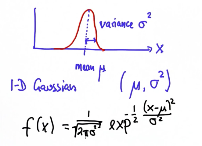
Larger the value of x and smaller the value of sigma, the better. Cause it will maximize the value of the outcome, which gives a narrower gaussian. And narrow gaussian with low sigma represents a more confident distribution, and that's what we want for accident-prone decision making.

Concepts

Same approach of sense (measurement) and move (motion) as Monte Carlo localization.

• Sense - Product, Bayesian Rule
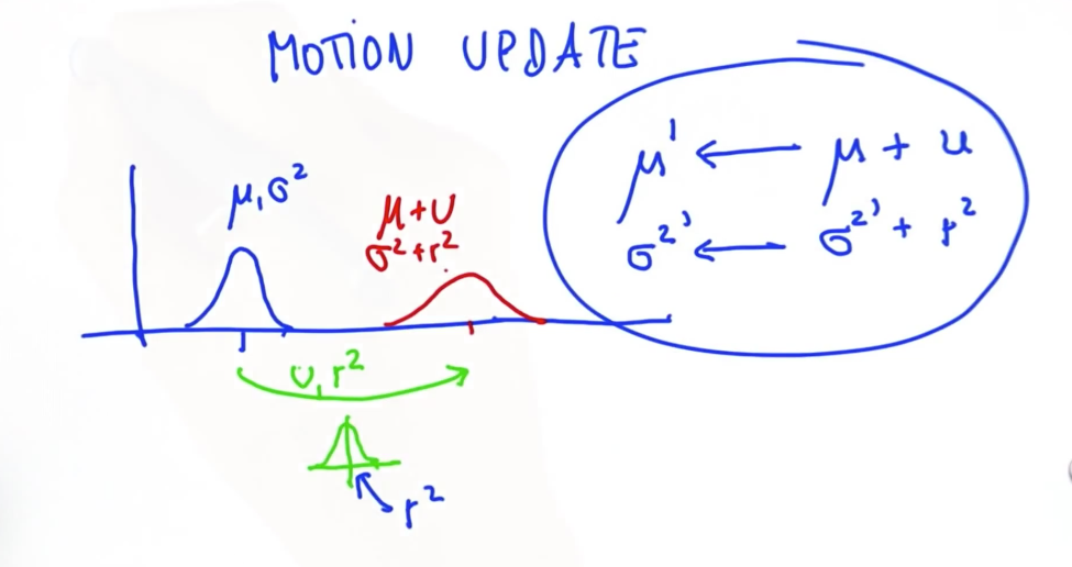
• Move - Convolution, Total Probability

Think of mean as the bottom center point of the gaussian and sigma as the half-width.

• As the gaussian becomes more and more peaky/certain with subsequent measurement/motions, it will pull the subsequent mean towards the peaky one.

(And every new mean will exist in between the last two means?)

• So think of mean as the actual location and covariance as the certainty.

Sensing

Two gaussians, representing prior and measurement. The prior gaussian would be a result of the last motion telling where we should be, and the measurement would be a result of, well, measurement/sense from the sensor telling where we are. And the final resulting gaussian would be a reconciliation of the two using the bayesian rule. Unlike the Monte Carlo approach where we derive a posterior probability, here we would derive a posterior mean and covariance of the resulting gaussian.

Mean -

Covariance -

And the following is how we get the posterior gaussian

$\mu^{\prime} = \frac{1}{\sigma^2 + r^2} [r^2\mu + \sigma^2\gamma]$

$\sigma^{2^{\prime}} = \frac{1}{\frac{1}{\sigma^2} + \frac{1}{r^2}}$

Don't be confused with the squares, the covariances already come as squares

Some intuitive things

Can also be derived from above formula

• If there are two gaussians far apart with the same covariance (sigma), then the new mean will be right in the midpoint of the two means. You can verify this by plugging into the formula. Also the new gaussian will have the covariance that is half of the previous gaussian, so it will be more peaky and confident.

Moving

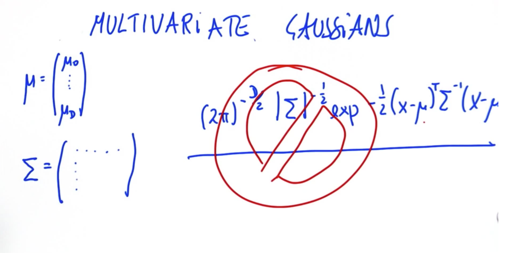
Multivariate Gaussian

For higher than 1D Can't use the above formula since they are only for 1D

Tips

• When initializing P covariance matrix for the first time, initialize the diagonals to the best of your ability, and the kalman filter should populate the non-diagonals over time as you measure and predict. Almost never want to initiate the diagonal to zero since that would indicate a perfect error-free measurement. So make sure to incorporate something by looking at the physics of things - how big is the overall field, what can the biggest/common measurement mistake be and square that so you get sigma square (standard deviation is just sigma)
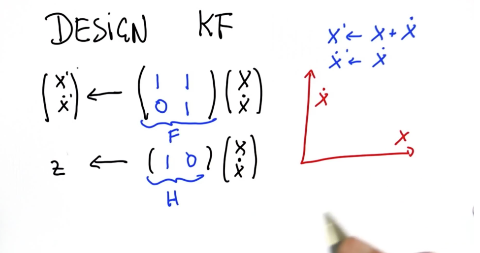
• Motion vector/ Control Vector/ Mu would be populated if you know you would be changing things that affect motion. Something like asteroids aren't controlled by you, so there'd be no Mu affecting things. But for a robot that you're moving, your dictating the motion (turn left, turn right), and you are expecting to see a certain behavior. That behavior is what is embedded in to the motion vector.
• If you don't use enough state variables (for example, you only use velocity when you should've also used acceleration to better tune the kalman filter), you want to add the Q i.e. covariance matrix that models the uncertainty in the state dynamics model - as shown in the tutorial by Leo.